
Copula Functions, R, and the Financial Crisis
[This article was first published on Econometric Sense, and kindly contributed to R-bloggers]. (You can report issue about the content on this page here)
Want to share your content on R-bloggers? click here if you have a blog, or here if you don't.
From: In defense of the Gaussian copula, The EconomistWant to share your content on R-bloggers? click here if you have a blog, or here if you don't.
“The Gaussian copula provided a convenient way to describe a relationship that held under particular conditions. But it was fed data that reflected a period when housing prices were not correlated to the extent that they turned out to be when the housing bubble popped.”
Decisions about risk, leverage, and asset prices would very likely become more correlated in an environment of centrally planned interest rates than under ‘normal’ conditions.
Simulations using copulas can be implemented in R. I’m not an expert in this, but thanks to the reference Enjoy the Joy of Copulas: With a Package copula I have at least gained a better understanding of copulas.
A copula can be defined as a multivariate distribution with marginals that are uniform over the unit interval (0,1). Copula functions can be used to simulate a dependence structure independently from the marginal distributions.
Based on Sklar’s theorem the multivariate distribution F can be represented by copula C as follows:
F(x1…xp) = C{ F1(x1),…, Fp(xp)}
where each Fi(xi) is a uniform marginal distribution.
Various functional forms for copula functions exist, each based on different assumptions about the dependence structure of the underlying variables. Using R, I have simulated data based on 3 different copula formulations (for 2 variable cases) and produced scatter plots for each.
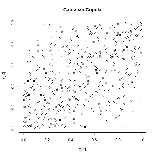
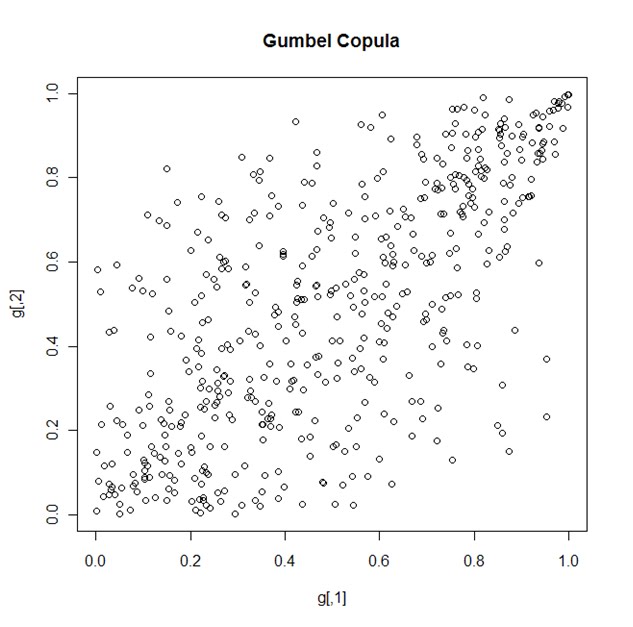
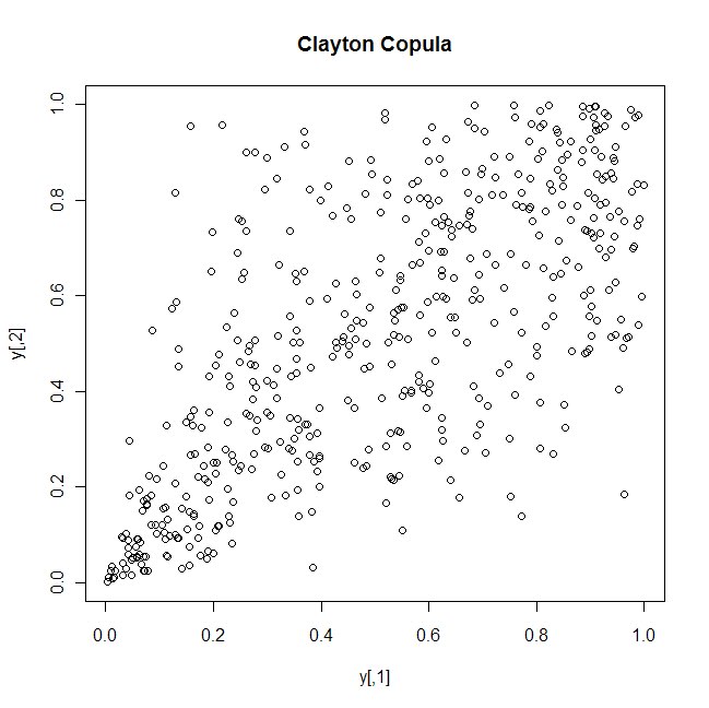
A mentioned in the Economist article at the beginning of this post, the gaussian copula was used widely before the housing crisis to simulate the dependence between housing prices in various geographic areas of the country. Looking at the plot for the gaussian copula above, it can be seen that extreme events (very high values of X1 and X2 or very low values of X1 and X2) seem very weakly correlated. The dependencies between X1 and X2 are very weak. We can see that with the Gumbel copula, extreme events (very high values of g1 and g2) are more correlated, while with the Clayton copula, extreme events (very low y1 and y2) are more correlated.
How might this relate to the financial crisis specifically? In The Role of Copulas in the Housing Crisis, Zimmer states:
“Due to its simplicity and familiarity, the Gaussian copula is popular in the calculation of risk in collaterized debt obligations. But the Gaussian copula imposes asymptotic independence such that extreme events appear to be unrelated. This restriction might be innocuous in normal times, but during extreme events, such as the housing crisis, the Gaussian copula might be inappropriate”
In the paper a mixture of Clayton and Gumbel copulas is investigated as an alternative to using the Gaussian copula.
The R code that I used to create the plots above, in addition to some additional plots, can be found below. I also highly recommend JD Long’s blog post Stochastic Simulation with Copula Functions in R.
References:
The Role of Copulas in the Housing Crisis. The Review of Economics and Statistics. Accepted for publication. Posted Online December 8, 2010. David M. Zimmer. Western Kentucky University.
Enjoy the Joy of Copulas: With a Package copula. Journal of Statistical Software Oct 2007, vol 21 Issue 1.
R-CODE
# *------------------------------------------------------------------
# | PROGRAM NAME: R_COPULA_BASIC
# | DATE: 1/25/11
# | CREATED BY: Matt Bogard
# | PROJECT FILE: P:\R  Code References\SIMULATION
# *----------------------------------------------------------------
# | PURPOSE:    copula graphics
# |
# *------------------------------------------------------------------
# | COMMENTS:
# |
# |  1: REFERENCES:  Emjoy the Joy of Copulas: With a Package copula
# |     Journal of Statistical Software Oct 2007, vol 21 Issue 1
# |      http://www.jstatsoft.org/v21/i04/paper
# |  2:
# |  3:
# |*------------------------------------------------------------------
# | DATA USED:
# |
# |
# |*------------------------------------------------------------------
# | CONTENTS:
# |
# |  PART 1:
# |  PART 2:
# |  PART 3:
# *-----------------------------------------------------------------
# | UPDATES:
# |
# |
# *------------------------------------------------------------------


library("copula")
set.seed(1)

# *------------------------------------------------------------------
# |
# |scatterplots
# |
# |
# *-----------------------------------------------------------------


# normal (Gausian?) Copula

norm.cop <- normalCopula(2, dim =3)
norm.cop
x <- rcopula(norm.cop, 500)
plot(x)
title("Gaussian Copula")

# Clayton Copula

clayton.cop <- claytonCopula(2, dim = 2)
clayton.cop
y <- rcopula(clayton.cop,500)
plot(y)
title("Clayton Copula")

# Frank Copula

frank.cop <- frankCopula(2, dim = 2)
frank.cop
f <- rcopula(frank.cop,500)
plot(f)
title("Frank Copula")


# Gumbel Copula

gumbel.cop <- gumbelCopula(2, dim = 2)
gumbel.cop
g <- rcopula(gumbel.cop,500)
plot(g)
title('Gumbel Copula')

# *------------------------------------------------------------------
# |
# |  contour plots
# |
# |
# *-----------------------------------------------------------------


# clayton copula contour
myMvd1 <- mvdc(copula = archmCopula(family = "clayton", param = 2),
margins = c("norm", "norm"), paramMargins = list(list(mean = 0,
sd = 1), list(mean = 0, sd = 1)))

contour(myMvd1, dmvdc, xlim = c(-3, 3), ylim = c(-3, 3))
title("Clayton Copula")

# frank copula contour
myMvd2 <- mvdc(copula = archmCopula(family = "frank", param = 5.736),
margins = c("norm", "norm"), paramMargins = list(list(mean = 0,
sd = 1), list(mean = 0, sd = 1)))

contour(myMvd2, dmvdc, xlim = c(-3, 3), ylim = c(-3, 3))
title("Frank Copula")

# gumbel copula
myMvd3 <- mvdc(copula = archmCopula(family = "gumbel", param = 2),
margins = c("norm", "norm"), paramMargins = list(list(mean = 0,
sd = 1), list(mean = 0, sd = 1)))

contour(myMvd3, dmvdc, xlim = c(-3, 3), ylim = c(-3, 3))
title("Gumbel Copula")To leave a comment for the author, please follow the link and comment on their blog: Econometric Sense.
R-bloggers.com offers daily e-mail updates about R news and tutorials about learning R and many other topics. Click here if you're looking to post or find an R/data-science job.
Want to share your content on R-bloggers? click here if you have a blog, or here if you don't.