Yesterday I surfed the web looking for 3D wireframe examples to explain linear models in class. I stumbled across this site where animated 3D wireframe plots are outputted by SAS.  Below I did something similar in R. This post shows the few steps of how to create an animated .gif file using R and ImageMagick. Here I assume that you have ImageMagick installed on your computer. As far as I know it is also possible to produce animated .gif files using R only, e.g. with write.gif() from the caTools package. But using ImageMagick is straighforward, gives you control over the conversion and .gif production and is the free standard program for conversion.

First a simple countdown example. To be sure not to overwrite anything I will create a new folder and set the working directory to the new folder.

dir.create("examples")
setwd("examples")

# example 1: simple animated countdown from 10 to "GO!".
png(file="example%02d.png", width=200, height=200)
  for (i in c(10:1, "G0!")){
    plot.new()
    text(.5, .5, i, cex = 6)
  }
dev.off()

# convert the .png files to one .gif file using ImageMagick. 
# The system() function executes the command as if it was done
# in the terminal. the -delay flag sets the time between showing
# the frames, i.e. the speed of the animation.
system("convert -delay 80 *.png example_1.gif")

# to not leave the directory with the single jpeg files
# I remove them.
file.remove(list.files(pattern=".png"))

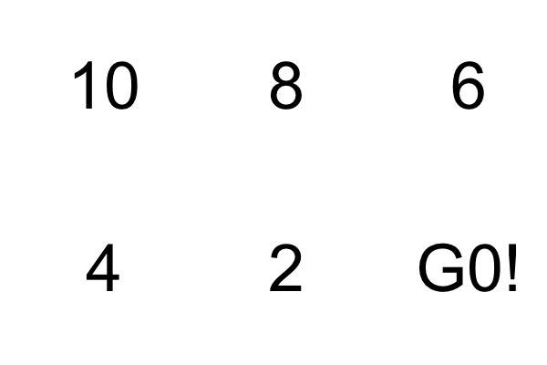
Above a loop is used to do the plotting. A new .png file for each plot is created automatically. The "%02d" part in the  filenamepart is a placeholder here for a two character counter (01,02 etc.). So we do not have to hard-code the filename each time.

Now I want a linear model to be visualized as a 3d mesh.  A 3D surface can easily be plotted using the wireframe() function from the lattice package (or other functions available in R; also see the rgl package for rotatable 3D output).

library(lattice)
b0 <- 10
b1 <- .5
b2 <- .3
g <- expand.grid(x = 1:20, y = 1:20)
g$z <- b0 + b1*g$x + b2*g$y
wireframe(z ~ x * y, data = g)

# to rotate the plot
wireframe(z ~ x * y, data = g,
          screen = list(z = 10, x = -60))

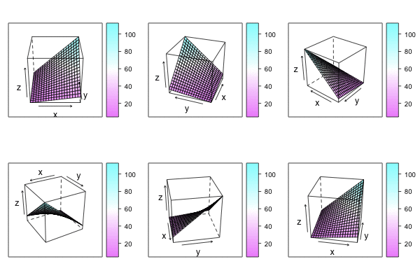
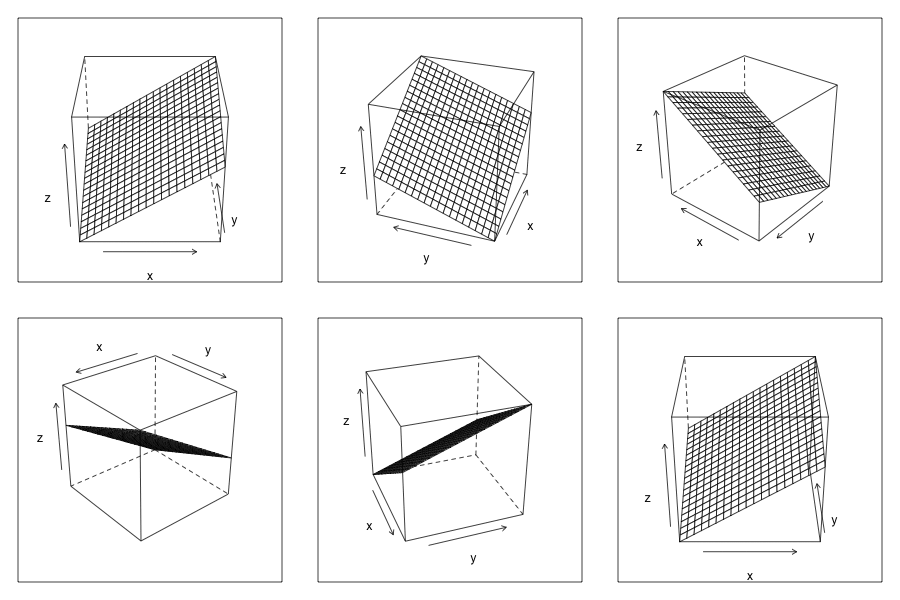
Now let’s create multiple files while changing the rotation angle. Note that wireframe() returns a trellis object which needs to be printed explicitly here using print(). As the code below produces over 150 images and merges them into one .gif file note that this may take a minute or two.

# example 2
png(file="example%03d.png", width=300, heigh=300)
  for (i in seq(0, 350 , 10)){
    print(wireframe(z ~ x * y, data = g,
              screen = list(z = i, x = -60)))
  }
dev.off()
# convert pngs to one gif using ImageMagick
system("convert -delay 40 *.png example_2_reduced.gif")

# cleaning up
file.remove(list.files(pattern=".png"))

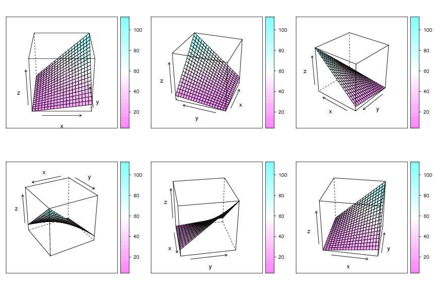
Now I want the same as above but for a model with an interaction and I want to make the plot a bit more pretty. This time I use .pdf as output file. This is just to demonstrate that other formats than .png can be used. Note that the "%02d" part of the filename has disappeared as I only create one .pdf file with multiple pages, not multiple .pdf files.

# example 3
b0 <- 10
b1 <- .5
b2 <- .3
int12 <- .2
g <- expand.grid(x = 1:20, y = 1:20)
g$z <- b0 + b1*g$x + b2*g$y + int12*g$x*g$y

pdf(file="example_3.pdf", width=4, height=4)
  for (i in seq(0, 350 ,10)){
    print(wireframe(z ~ x * y, data = g,
              screen = list(z = i, x = -60),
              drape=TRUE))
  }
dev.off()
# convert pdf to gif using ImageMagick
system("convert -delay 40 *.pdf example_3_reduced.gif")
# cleaning up
file.remove(list.files(pattern=".pdf"))

The last example is a visual comparison of the interaction and a non-interaction model. Here we now have the models on the same scale. Before I did not specify the scale limits.

# example 4
b0 <- 10
b1 <- .5
b2 <- .3
int12 <- .2
g <- expand.grid(x = 1:20, y = 1:20)
z <- c( b0 + b1*g$x + b2*g$y,
        b0 + b1*g$x + b2*g$y + int12*g$x*g$y)
g <-rbind(g, g)
g$z <- z
g$group <- gl(2, nrow(g)/2, labels=c("interaction", "no interaction"))

png(file="example%03d.png", width=300, height=300)
  for (i in seq(0, 350 ,10)){
    print(wireframe(z ~ x * y, data = g, groups=group,
              screen = list(z = i, x = -60)))
  }
dev.off()
# convert pngs to one gif using ImageMagick
system("convert -delay 40 *.png example_4.gif")

# cleaning up
file.remove(list.files(pattern=".png"))

Above I chose a small image size (300 x 300 pts). Smaller steps for rotation and a bigger picture size increases file sizes for examples 2, 3 and 4 to 3-5mb which is far too big for a web format. I am not familiar with image optimization and I suppose a smaller file sizes for the .gif file can easily be achieved by some optimization flags in ImageMagick. Any hints are welcome!