
Using Decision Trees to Predict Infant Birth Weights
Want to share your content on R-bloggers? click here if you have a blog, or here if you don't.
In this article, I will show you how to use decision trees to predict whether the birth weights of infants will be low or not. We will use the birthwt data from the MASS library.
What is a decision tree?
A decision tree is an algorithm that builds a flowchart like graph to illustrate the possible outcomes of a decision. To build the tree, the algorithm first finds the variable that does the best job of separating the data into two groups. Then, it repeats the above step with the other variables. This results in a tree graph, where each split represents a decision. The algorithm chooses the splits such that the maximum number of observations are classified correctly. The biggest advantage of a decision tree is that it is really intuitive and can be understood even by people with no experience in the field.
For example, a classification tree showing the survival of passengers of the Titanic is as follows (source: Wikipedia):
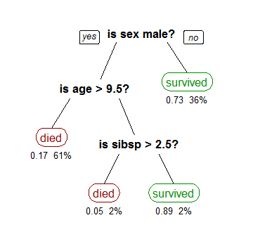
The numbers under the node represent the probability of survival, and the percentage of observations that fall into that category. The first node on the right shows that 73% of the females survived, and females represented 36% of the total observations in the dataset.
Exploring the data
We will need the MASS and rpart libraries for this. Let’s load up the data, and look at it.
library(MASS)
library(rpart)
head(birthwt)
   low age lwt race smoke ptl ht ui ftv  bwt
85   0  19 182    2     0   0  0  1   0 2523
86   0  33 155    3     0   0  0  0   3 2551
87   0  20 105    1     1   0  0  0   1 2557
88   0  21 108    1     1   0  0  1   2 2594
89   0  18 107    1     1   0  0  1   0 2600
91   0  21 124    3     0   0  0  0   0 2622
From the help file,
- low – indicator of whether the birth weight is less than 2.5kg
- age – mother’s age in year
- lwt – mother’s weight in pounds at last menstrual period
- race – mother’s race (1 = white, 2 = black, white = other)
- smoke – smoking status during pregnancy
- ptl – number of previous premature labours
- ht – history of hypertension
- ui – presence of uterine irritability
- ftv – number of physician visits during the first trimester
- bwt – birth weight in grams
Let’s look at the distribution of infant weights:
hist(birthwt$bwt)
This gives us the following histogram:
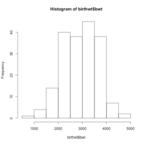
Most of the infants weigh between 2kg and 4kg.
Now, let us look at the number of infants born with low weight.
table(birthwt$low)
  0   1
130  59
This means that there are 130 infants weighing more than 2.5kg and 59 infants weighing less than 2.5kg. If we just guessed the most common occurrence (> 2.5kg), our accuracy would be 130 / (130 + 59) = 68.78%. Let’s see if we can improve upon this by building a prediction model.
Building the model
In the dataset, all the variables are stored as numeric. Before we build our model, we need to convert the categorical variables to factor.
cols <- c('low', 'race', 'smoke', 'ht', 'ui')
birthwt[cols] <- lapply(birthwt[cols], as.factor)
Next, let us split our dataset so that we have a training set and a testing set.
set.seed(1)
train <- sample(1:nrow(birthwt), 0.75 * nrow(birthwt))
Now, let us build the model. We will use the rpart function for this.
birthwtTree <- rpart(low ~ . - bwt, data = birthwt[train, ], method = 'class')
Since low = bwt <= 2.5, we exclude bwt from the model, and since it is a classification task, we specify method = 'class'. Let’s take a look at the tree.
plot(birthwtTree)
text(birthwtTree, pretty = 0)
This is what it looks like:
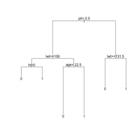
This means that if the mother has had one or more premature labours previously, and her weight at the last menstrual period was equal to or higher than 131.5 pounds, then the infant is likely to be born with low weight. The other nodes can be interpreted similarly.
We can get a more detailed, textual summary of the tree as follows:
summary(birthwtTree)
Since the summary is rather detailed and long, I will not paste it here. It contains more information about the number of observations at each node, and also their probabilities.
Let us now see how the model performs on the test set.
birthwtPred <- predict(birthwtTree, birthwt[-train, ], type = 'class')
table(birthwtPred, birthwt[-train, ]$low)
birthwtPred  0  1
          0 31 10
          1  2  5
Hence, the accuracy is (31 + 5) / (31 + 5 + 2 + 10) = 75%! Not bad, huh? The accuracy can further be improved by techniques such as bagging and random forests. If you are more interested in learning about these, and the mathematics behind the decision tree, I highly suggest referring to Introduction to Statistical Learning.
That brings us to the end of the article. I hope you enjoyed it and found it useful. If you have any questions or feedback, feel free to leave a comment or reach out to me on Twitter!
R-bloggers.com offers daily e-mail updates about R news and tutorials about learning R and many other topics. Click here if you're looking to post or find an R/data-science job.
Want to share your content on R-bloggers? click here if you have a blog, or here if you don't.