
The Generalized Lambda Distribution and GLDEX Package: Fitting Financial Return Data
Want to share your content on R-bloggers? click here if you have a blog, or here if you don't.
by Daniel Hanson, with contributions by Steve Su (author of the GLDEX package). Part 1 of a series.
Introduction
As most readers are well aware, market return data tends to have heavier tails than that which can be captured by a normal distribution; furthermore, skewness will not be captured either. For this reason, a four parameter distribution such as the Generalized Lambda Distribution (GLD) can give us a more realistic representation of the behavior of market returns, including a more accurate measure of expected loss in risk management applications as compared to the normal distribution.
This is not to say that the normal distribution should be thrown in the dustbin, as the underlying stochastic calculus, based on Brownian Motion, remains a very convenient tool in modeling derivatives pricing and risk exposures (see earlier blog article here), but like all modeling methods, it has its strengths and weaknesses.
As noted in the book Financial Risk Modelling and Portfolio Optimization with R (Pfaff, Ch 6: Suitable distributions for returns) (publisher information provided here), the GLD is one of the recommended distributions to consider in order “to model not just the tail behavior of the losses, but the entire return distribution. This need arises when, for example, returns have to be sampled for Monte Carlo type applications.” The author provides descriptions and examples of several R packages freely available on the CRAN website, namely Davies, fBasics, gld, and lmomco. Another package, also freely available on CRAN, is the GLDEX package, which is the package we will use in the current article. It contains a rich offering of functions and is well documented. In addition, the author of the GLDEX package, Dr Steve Su, has kindly provided assistance in the writing of this article. He has also published a very useful and related article in the Journal of Statistical Software (JSS) (2007), to which we will refer in the discussion below.
Brief Background on the GLD
The four parameters of the GLD are, not surprisingly, λ1, λ2, λ3, and λ4. Without going into theoretical details, suffice it to say that λ1 and λ2 are measures of location and scale respectively, while the skewness and kurtosis of the distribution are determined by λ3 and λ4.
Furthermore, there are two forms of the GLD that are implemented in GLDEX, namely those of Ramberg and Schmeiser (1974), and Freimer, Mudholkar, Kollia, and Lin (1988). These are commonly abbreviated as RS and FMKL. As the FMKL form is the more modern of the two, we will focus on it in the discussion that follows. An additional reference frequently cited in the literature related to the GLD in finance is the paper by Chalabi, Scott, and Wurtz, freely available here on the rmetrics website.
Fitting a Time Series of Financial Returns to the GLD
As Steve Su points out in his 2007 JSS article on the GLDEX package (see link above), there are three basic steps that are useful in determining the quality of the GLD fit. The first two, as we shall see, can be competing objectives in determining the fit. The GLDEX package provides functionality for each.
- Comparing the mean, variance, skewness and kurtosis of the fitted distribution with the empirical data
- The Komogorov-Smirnoff (KS) resample test and goodness of fit
- Graphical outputs
Remark: The list of options has been presented here in opposite order of that in the JSS article in order to assist in the development of the discussion, as we shall see.
Market Returns Data
Let’s first obtain some market data to use. The Wilshire 5000 index is commonly used as a measure of the total US equity market — comprising large, medium, and small cap stocks — so we call once again upon our old friend the quantmod package to access the past 20 years of daily closing prices of the Vanguard Total Stock Market Index Fund (VTSMX).
require(quantmod) # quantmod package must be installed
getSymbols(“VTSMX”, from = “1994-09-01”)
VTSMX.Close <- VTSMX[,4] # Closing prices
VTSMX.vector <- as.vector(VTSMX.Close)
# Calculate log returns
Wilsh5000 <- diff(log(VTSMX.vector), lag = 1)
Wilsh5000 <- 100 * Wilsh5000[-1] # Remove the NA in the first position,
# and put in percent format
Method of Moments
Appealing to step (1) above, the following function uses the FMKL form to fit the data to a GLD with the method of moments,
wshLambdaMM <- fun.RMFMKL.mm(Wilsh5000)
This returns the estimated values of λ1, λ2, λ3, and λ4 in the vector wshLambdaMM :
[1] 0.04882924 1.98442097 -0.16423899 -0.13470102
Remark: Warning messages such as the following may occur when running this function:
Warning messages:
1: In beta(a, b) : NaNs produced
2: In beta(a, b) : NaNs produced
…
These may be ignored.
We can then compare the four moments of the fitted distribution with those of the market data using the following functions respectively:
# Moments of fitted distribution:
fun.theo.mv.gld(wshLambdaMM[1], wshLambdaMM[2], wshLambdaMM[3], wshLambdaMM[4],
param = “fmkl”, normalise=”Y”)
# Results:
# mean variance skewness kurtosis
# 0.02824672 1.50214919 -0.30413445 7.8210743
# Moments of Wilshire 5000 market returns:
fun.moments.r(Wilsh5000,normalise=”Y”) # normalise=”Y” — subtracts the 3
# from the normal dist value.
# Results:
# mean variance skewness kurtosis
# 0.02824676 1.50214916 -0.30413445 7.82107430
We’re basically spot-on here, and things are looking pretty good; however, we haven’t looked at a goodness of fit test yet, and unfortunately, this will tell a different story. We will first look at the Komogorov-Smirnoff (KS) resample test, as shown in the 2007 JSS article. The test is based on the sample statistic Kolmogorov-Smirnoff Distance (D) between the data in the sample and the fitted distribution. The null hypothesis is, simply speaking, that the sample data is drawn from the same distribution as the fitted distribution.
The function here, from the GLDEX package, samples a proportion (default = 90%) of the data and fitted distribution and calculates the KS test p-value 1000 times (no.test argument), and returns the number of times that the p-value is not significant. The higher the number, the more confident we can be that the fitted distribution is reasonable.
fun.diag.ks.g(result = wshLambdaMM, data = Wilsh5000, no.test = 1000,
param = “fmkl”)
Our result here is 53/1000, which suggests that we’re pretty way off. A more recent addition to the GLDEX package that was not available at the time the related 2007 JSS article was written is the following:
ks.gof(Wilsh5000, “pgl”, wshLambdaMM, param=”fmkl”)
where pgl is the GLD distribution function included in the GLDEX package (the analog of the pnorm normal distribution function included in Base R).
With a p-value of 1.912e-05, it is pretty safe to reject the hypothesis that the sample data is drawn from the fitted distribution.
Method of Maximum Likelihood (ML)
As Steve Su points out in his JSS article, “The maximum likelihood estimation is usually the preferred method” for “providing definite fits to a data set using the GLD”. The function in the GLDEX package, again for the FKML parameterization, is
wshLambdaML = fun.RMFMKL.ml(Wilsh5000)
Checking our goodness of fit tests,
fun.diag.ks.g(result = wshLambdaML, data = Wilsh5000, no.test = 1000, param = “fmkl”)
We get a result of 825/1000, and for
ks.gof(Wilsh5000,”pgl”, wshLambdaML, param=”fmkl”)
we get D = 0.0151, p-value = 0.2
This p-value, while not spectacular, is far better than what we saw for the method of moments case, and the KS resample test is also much more convincing. But now, the “bad news”: if we look at the four moments of the ML fit,
fun.theo.mv.gld(wshLambdaML[1], wshLambdaML[2], wshLambdaML[3],
wshLambdaML[4], param = “fmkl”, normalise=”Y”)
we get
# mean variance skewness kurtosis
# 0.02850058 1.64456695 -2.13494680 NA
While the mean and variance are reasonably close to their empirical counterparts, skewness is off by about 60%, and kurtosis can’t be determined by the algorithm.
Graphical Comparison of Method of Moments and Maximum Likelihood
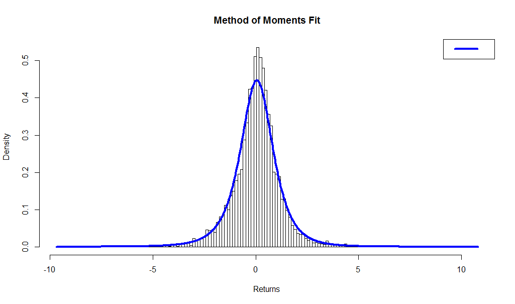
Now, invoking step 3, let’s compare the plots resulting from the two different methods, using the fun.plot.fit(.) function provided in the GLDEX package, by overlaying the pdf curve of the fitted distribution on top of the histogram of the returns data. In order to assure a meaningful plot, however, we should first determine the optimal number of bins in the histogram using the Freedman-Diaconis Rule with the following R function:
bins <- nclass.FD(Wilsh5000) # We get 158
Then, set nclass = bins into the plotting function in the GLDEX package:
# Method of Moments
fun.plot.fit(fit.obj = wshLambdaMM, data = Wilsh5000, nclass = bins,
param = “fmkl”,
xlab = “Returns”, main = “Method of Moments Fit”)
# Method of Maximum Likelihood
fun.plot.fit(fit.obj = wshLambdaML, data = Wilsh5000,
nclass = bins, param = “fkml”,
xlab = “Returns”, main = “Method of Maximum Likelihood”)
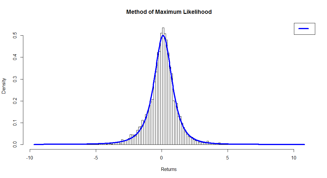
Visual inspection of the plots is consistent with our findings above, that the method of maximum likelihood results in a better fit of the data than the method of moments, despite the fact that the moments line up almost exactly in the case of the former.
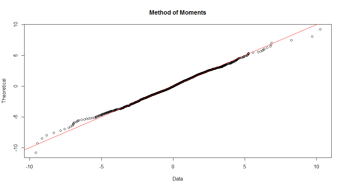
One more set of plots that one should inspect is the set of quantile (“QQ”) plots:
qqplot.gld(fit=wshLambdaMM,data=Wilsh5000,param=”fkml”, type = “str.qqplot”,
main = “Method of Moments”)
qqplot.gld(fit=wshLambdaML,data=Wilsh5000,param=”fkml”, type = “str.qqplot”,
main = “Method of Maximum Likelihood”)
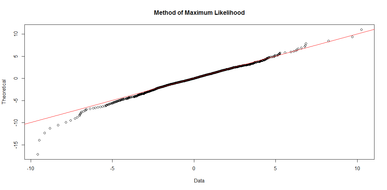
Now, if we were to look at these two plots in a vacuum, so to speak, with none of the other prior information available, there is a good case to be made that the QQ plot for Method of Moments might indicate a better fit. However, note that at about -4 along the horizontal (empirical data) axis, the plotted points start to drift above the line indicating where the horizontal and vertical axis values are equal. This implies that our fit is underestimating market losses as we move out toward the left tail of the distribution. The QQ plot for Maximum Likelihood is more conservative, erring on the side of caution with the fitted distribution indicating an increased risk of greater loss than the Method of Moments fit. As Steve Su puts it, the general recommendation is to look at the QQ plot and KS test results together, to determine the goodness of fit. The QQ plot alone, however, is not a fail-proof method.
Conclusion
We have seen, using R and the GLDEX package, how a four parameter distribution such as the Generalized Lambda Distribution can be used to fit a distribution to market data. While the Method of Moments as a fitting algorithm is highly appealing due to its preserving the moments of the empirical distribution, we sacrifice goodness of fit that can be obtained by using the Method of Maximum Likelihood.
In our next article, we will look at an alternative GLD fitting method know as the Method of L-Moments as a compromise between the two methods discussed here, and then conclude with a comparison with the normal distribution, which will exhibit quite clearly the advantages of the GLD when it comes to fitting financial returns data.
Very special thanks are due to Dr Steve Su for his contributions and guidance in presenting this topic.
R-bloggers.com offers daily e-mail updates about R news and tutorials about learning R and many other topics. Click here if you're looking to post or find an R/data-science job.
Want to share your content on R-bloggers? click here if you have a blog, or here if you don't.