
Poor man’s integration – a simulated visualization approach
Want to share your content on R-bloggers? click here if you have a blog, or here if you don't.
Every once in a while I encounter a problem that requires the use of calculus. This can be quite bothersome since my brain has refused over the years to retain any useful information related to calculus. Most of my formal training in the dark arts was completed in high school and has not been covered extensively in my post-graduate education. Fortunately, the times when I am required to use calculus are usually limited to the basics, e.g., integration and derivation. If you’re a regular reader of my blog, you’ll know that I often try to make life simpler through the use of R. The focus of this blog is the presentation of a function that can integrate an arbitrarily-defined curve using a less than quantitative approach, or what I like to call, poor man’s integration. If you are up to speed on the basics of calculus, you may recognize this approach as Monte Carlo integration. I have to credit Dr. James Forester (FWCB dept., UMN) for introducing me to this idea.
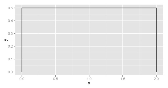
If you’re like me, you’ll need a bit of a refresher on the basics of integration. Simply put, the area underneath a curve, bounded by some x-values, can be obtained through integration. Most introductory calculus texts will illustrate this concept using a uniform distribution, such as:
= \left\{ \begin{array}{l l} 0.5 & \quad \textrm{if } 0 \leq x \leq 2 \\ 0 & \quad \textrm{otherwise} \end{array} \right.")
If we want to get the area of the curve between, for example 0.5 and 1.5, we find the area of the blue box:
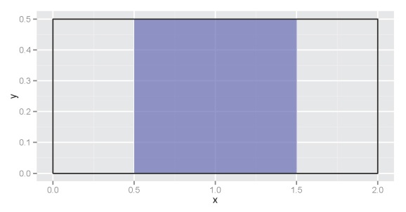
Going back to basic geometry, we know that this is the width (1.5-0.5) multiplied by the height (0.5-0), or 0.5. In calculus terms, this means we’ve integrated the uniform function with the definite integral from 0.5 to 1.5. Integration becomes more complicated with increasingly complex functions and we can’t use simple geometric equations to obtain an answer. For example, let’s define our function as:
= 1 + x^{2} \quad \textrm{for} {}-\infty < x < {}+\infty")
Now we want to integrate the function from -1 to 1 as follows:
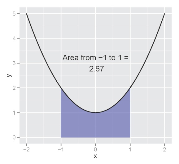
Using calculus to find the area:
dx & = & \int\limits_{{}-1}^{1} 1 + x^{2} dx \\ & = & \left( 1 + \frac{1}{3}1^{3} \right) - \left({}-1 + \frac{1}{3}\left({}-1\right)^{3} \right) \\ & = & 1.33 + 1.33 \\ & = & 2.67 \end{array}")
The integrated portion is the area of the curve from negative infinity to 1 minus the area from negative infinity to -1, where the area is determined based on the integrated form of the function, or the antiderivative. The integrate function in R can perform these calculations for you, so long as you define your function properly.
int.fun<-function(x) 1+x^2
integrate(int.fun,-1,1)
The integrate function will return the same value as above, with an indication of error for the estimate. The nice aspect about the integrate function is that it can return integral estimates if the antiderivative has no closed form solution. This is accomplished (from the help file) using ‘globally adaptive interval subdivision in connection with extrapolation by Wynn’s Epsilon algorithm, with the basic step being Gauss–Kronrod quadrature’. I’d rather take a cold shower than figure out what this means. However, I assume the integration involves summing the area of increasingly small polygons across the interval, something like this. The approach I describe here is similar except random points are placed in the interval, rather than columns. The number of points under the curve relative to total number of points is multiplied by the total area that the points cover. The integral estimation approximates the actual as the number of points approaches infinity. After creating this function, I realized that the integrate function can accomplish the same task. However, I’ve incorporated some plotting options for my function to illustrate how the integral is estimated.
Let’s start by creating an arbitrary model for integration. We’ll create random points and then approximate a line of best fit using the loess smoother.
set.seed(3)

x<-seq(1,10)
y<-runif(10,0,20)
dat<-data.frame(x,y)

model<-loess(y~x, data=dat)
The approximated loess model through our random points looks like this:
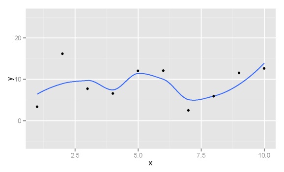
The antiderivative of the approximated model does not exist in a useful form since the loess function uses local fitting. We can use the integrate function to calculate the area under the curve. The integrate function requires as input a function that takes a numeric first argument and returns a numeric vector of the same length, so we have convert our model accordingly. We’ll approximate the definite integral from 4 to 8.
mod.fun<-function(x) predict(model,newdata=x)
integrate(mod.fun,4,8)
The function tells us that the area under the curve from 4 to 8 is 33.1073 with absolute error < 3.7e-13. Now we can compare this estimate to one obtained using my function. We'll import the mc.int function from Github.
require(devtools)
source_gist(5483807)
This function differs from integrate in a few key ways. The input is an R object model that has a predict (e.g., predict.lm) method, rather than an R function that returns a numeric vector the same length as the input. This is helpful because it eliminates the need to create your own prediction function for your model. Additionally, a plot is produced that shows the simulation data that were used to estimate the integral. Finally, the integration method uses randomly placed points rather than a polygon-based approach. I don’t know enough about integration to speak about the strength and weaknesses of either approach, but the point-based method is more straight-forward (in my opinion).
Let’s integrate our model from 4 to 8 using the mc.int function imported from Github.
mc.int(model,int=c(4,8),round.val=6)
The estimate returned by the function is 32.999005, which is very close to the estimate returned from integrate. The default behavior of mc.int is to return a plot showing the random points that were used to obtain the estimate:

All of the points in green were below the curve. The area where the points were randomly located (x = 4 to x = 8 and y=0 to y=14) was multiplied by the number of green points divided by the total number of points. The function has the following arguments:
mod.in |
fitted R model object, must have predict method |
int |
two-element numeric vector indicating interval for integration, integrates function across its range if none provided |
n |
numeric vector indicating number of random points to use, default 10000 |
int.base |
numeric vector indicating minimum y location for integration, default 0 |
plot |
logical value indicating if results should be plotted, default TRUE |
plot.pts |
logical value indicating if random points are plotted, default TRUE |
plot.poly |
logical value indicating if a polygon representing the integration region should be plotted, default TRUE |
cols |
three-element list indicating colors for points above curve, points below curve, and polygon, default ‘black’,'green’, and ‘blue’ |
round.val |
numeric vector indicating number of digits for rounding integration estimate, default 2 |
val |
logical value indicating if only the estimate is returned with no rounding, default TRUE |
Two characteristics of the function are worth noting. First, the integration estimate varies with the total number of points:
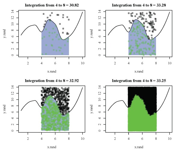
Second, the integration estimate changes if we run the function again with the same total number of points since the point locations are chosen randomly:

These two issues represent one drawback of the mc.int function because a measure of certainty is not provided with the integration estimate, unlike the integrate function. However, an evaluation of certainty for an integral with no closed form solution is difficult to obtain because the actual value is not known. Accordingly, we can test the accuracy and precision of the mc.int function to approximate an integral with a known value. For example, the integral of the standard normal distribution from -1.96 to 1.96 is 0.95.
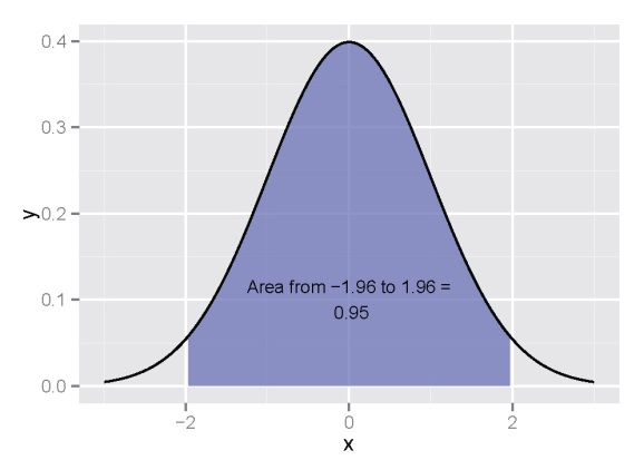
The mc.int function will only be useful if it produces estimates for this integral that are close to 0.95. These estimates should also exhibit minimal variation with repeated random estimates. To evaluate the function, we’ll test an increasing number of random points used to approximate the integral, in addition to repeated number of random estimates for each number of random points. This allows an evaluation of accuracy and precision. The following code evaluated number of random points from 10 to 1000 at intervals of 10, with 500 random samples for each interval. The code uses another function, mc.int.ex, imported from Github that is specific to the standard normal distribution.
#import mc.int.ex function for integration of standard normal
source_gist(5484425)

#get accuracy estimates from mc.int.ex
rand<-500
check.acc<-seq(10,1000,by=10)
mc.dat<-vector('list',length(check.acc))
names(mc.dat)<-check.acc
for(val in check.acc){
	out.int<-numeric(rand)
	for(i in 1:rand){
		cat('mc',val,'rand',i,'\n')
		out.int[i]<-mc.int.ex(n=val,val=T)
		flush.console()
		}
	mc.dat[[as.character(val)]]<-out.int
	}
The median integral estimate, as well as the 2.5th and 97.5th quantile values were obtained for the 500 random samples at each interval (i.e., a non-parametric bootstrap approach). Plotting the estimates as a function of number of random points shows that the integral estimate approaches 0.95 and the precision of the estimate increases with increasing number of points. In fact, an estimate of the integral with 10000 random points and 500 random samples is 0.950027 (0.9333885, 0.9648904).

The function is not perfect but it does provide a reasonable integration estimate if the sample size is sufficiently high. I don’t recommend using this function in place integrate, but it may be useful for visualizing an integration. Feel free to use/modify as you see fit. Cheers!

R-bloggers.com offers daily e-mail updates about R news and tutorials about learning R and many other topics. Click here if you're looking to post or find an R/data-science job.
Want to share your content on R-bloggers? click here if you have a blog, or here if you don't.