In marketing mix modelling you have to be very lucky not to run into problems with multicollinearity. It’s in the nature of marketing campaigns that everything tends to happen at once: the TV is supported by radio, both are timed to coincide with the relaunch of the website. One of the techniques that is often touted as a solution is ridge regression. However there is quite a bit of disagreement over whether this works. So I thought we’d just try it out with the simulated sales data I created in the last post.

In fact we’ll need to modify that data a little as we need a case of serious multicollinearity. I’ve adjusted the Tv campaigns to ensure that they always occur in the same winter months (not uncommon in marketing mix data) and I’ve added radio campaigns alongside the TV campaigns. Here is the modified code.

  #TV now coincides with winter. Carry over is dec, theta is dim, beta is ad_p,
  tv_grps<-rep(0,5*52)
  tv_grps[40:45]<-c(390,250,100,80,120,60)
  tv_grps[92:97]<-c(390,250,100,80,120,60)
  tv_grps[144:149]<-c(390,250,100,80,120,60)
  tv_grps[196:201]<-c(390,250,100,80,120,60)
  tv_grps[248:253]<-c(390,250,100,80,120,60)
  
  if (adstock_form==2){adstock<-adstock_calc_2(tv_grps, dec, dim)}
  else {adstock<-adstock_calc_1(tv_grps, dec, dim)}
  TV<-ad_p*adstock
  
  # Accompanying radio campaigns
  radio_spend<-rep(0,5*52)
  radio_spend[40:44]<-c(100, 100, 80, 80)
  radio_spend[92:95]<-c(100, 100, 80, 80)
  radio_spend[144:147]<-c(100, 100, 80)
  radio_spend[196:200]<-c(100, 100, 80, 80)
  radio_spend[248:253]<-c(100, 100, 80, 80, 80)
  radio<-radio_p*radio_spend

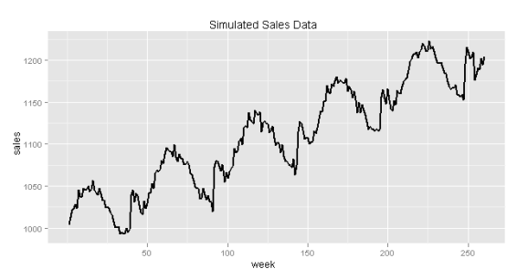
The sales data now looks like this:

The correlation matrix of the explanatory variables shows that we have serious multicollinearity issues even when only two variables are taken at a time.

 > cor(test[,c(2,4:6)])
                  temp radio_spend        week     adstock
temp         1.0000000 -0.41545174 -0.15593463 -0.47491671
radio_spend -0.4154517  1.00000000  0.09096521  0.90415219
week        -0.1559346  0.09096521  1.00000000  0.08048096
adstock     -0.4749167  0.90415219  0.08048096  1.00000000

What is this going to mean for the chances of recovering the parameters in our simulated data set? Well we know that even with heavy multicollinearity our estimates using linear regression are going to be unbiased; the problem is going to be their high variance.

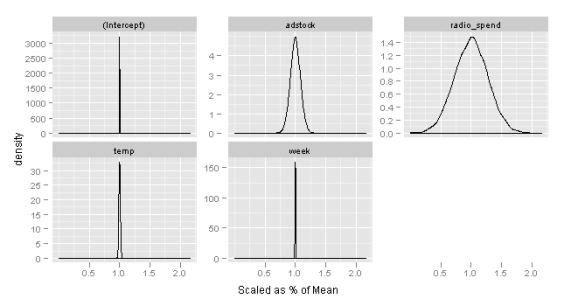
We can show this quite nicely by generating lots of examples of our sales data (always with the same parameters but allowing a different random draw each from the normally distributed error term) and plotting the distribution of the estimates arrived at using linear regression. (See Monte Carlo Simulation for more details about this kind of technique.)

}

You can see that on average the estimates for tv and radio are close to correct but the distributions are wide. So for any one instance of the data (which in real life is all we have) chances are that our estimate is quite wide of the mark. The data and plots are created using the following code:

 
coefs<-NA 
 
for (i in 1:10000){

   sim<-create_test_sets(base_p=1000,
                       trend_p=0.8,
                       season_p=4,
                       ad_p=30,
                       dim=100,
                       dec=0.3,
                       adstock_form=1,
                       radio_p=0.1,
                       error_std=5)
  lm_std<-lm(sales~week+temp+adstock+radio_spend, data=sim)
  coefs<-rbind(coefs,coef(lm_std))
  
}

col_means<-colMeans(coefs[-1,])
for_div<-matrix(rep(col_means,10000), nrow=10000, byrow=TRUE)
mean_div<-coefs[-1,]/for_div

m_coefs<-melt(mean_div)
ggplot(data=m_coefs, aes(x=value))+geom_density()+facet_wrap(~X2, scales="free_y") + scale_x_continuous('Scaled as % of Mean') 
 

What does ridge regression do to fix this? Ridge regression is best explained using a concept more familiar in machine learning and data mining: the bias-variance trade off. The idea is that you will often achieve better predictions (or estimates) if you are prepared to swap a bit of unbiasedness for much less variance. In other words the average of your predictions will no longer converge on the right answer but any one prediction is likely to be much closer.

In ridge regression we have a parameter lambda that controls the bias-variance trade off. As lambda increases our estimates get more biased but their variance increases. Cross-validation (another machine learning technique) is used to estimate the best possible setting of lambda.

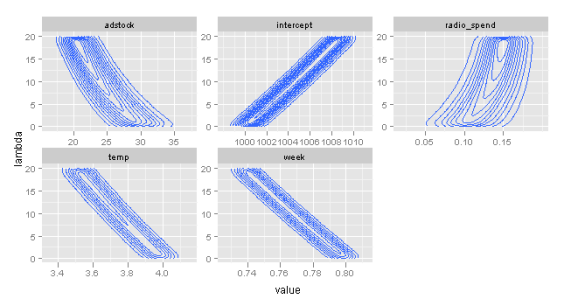
So let’s see if ridge regression can help us with the multicolinearity in our marketing mix data. What we hope to see is a decent reduction in variance but not at too high a price in bias. The code below simulates the distribution of the ridge regression estimates of the parameters for increasing values of lambda.

 
library(MASS)
 
for (i in 1:1000){

   sim<-create_test_sets(base_p=1000,
                       trend_p=0.8,
                       season_p=4,
                       ad_p=30,
                       dim=100,
                       dec=0.3,
                       adstock_form=1,
                       radio_p=0.1,
                       error_std=5)
  lm_rg<-lm.ridge(sales~week+temp+adstock+radio_spend, data=sim, lambda = seq(0,20,0.5))
  if (i==1){coefs_rg<-coef(lm_rg)}
  else {coefs_rg<-rbind(coefs_rg,coef(lm_rg))}
  
}
 
colnames(coefs_rg)[1]<-"intercept"
 
m_coefs_rg<-melt(coefs_rg)
  
names(m_coefs_rg)<-c("lambda", "variable", "value")

ggplot(data=m_coefs_rg, aes(x=value, y=lambda))+geom_density2d()+facet_wrap(~variable, scales="free")

The results are not encouraging. Variance decreases slightly for tv and radio however the cost in bias is far too high.

I’m aware that this by no means proves that ridge regression is never a solution for marketing mix data but it does at least show that it is not always the solution and I’m inclined to think that if it doesn’t work in a simple situation like this then it doesn’t work very often.

However I might try varying the parameters for the simulated data set to see if there are some settings where it looks more promising.

Still, for now, I won’t be recommending it as a solution to multicollinearity in marketing mix models.

A good explanation of ridge regression can be found in this post