
Major League Baseball run scoring trends with R’s Lahman package
[This article was first published on Bayes Ball, and kindly contributed to R-bloggers]. (You can report issue about the content on this page here)
Want to share your content on R-bloggers? click here if you have a blog, or here if you don't.
The statistical software R has an ever-expanding array of packages that provide pre-programmed functions and datasets. One such package is named Lahman, bundling the contents of the Lahman database into a quick-and-easy resource for R users. In addition to the data tables, the package resources also contain a variety of analyses and graphics undertaken using the package, providing some examples of how the package can be used.Want to share your content on R-bloggers? click here if you have a blog, or here if you don't.
Full disclosure: I am now one of the Lahman package project members.
This is my first blog post using the Lahman package, and as a first step I will simply recreate the league run scoring trends graphs that I generated previously. Originally, I had used data from Baseball Reference, for the simple reason that the Lahman database does not, in its source form, contain any league-level aggregations.
The process for loading the Lahman package is as simple as any other R package; this simplicity is even greater if you are using an IDE such as RStudio. Once loaded, you have access to all the tables in the database, without any of the futzing that is sometimes required in tidying up a raw flat file (I find that variable names are sometimes lost or changed in translation).
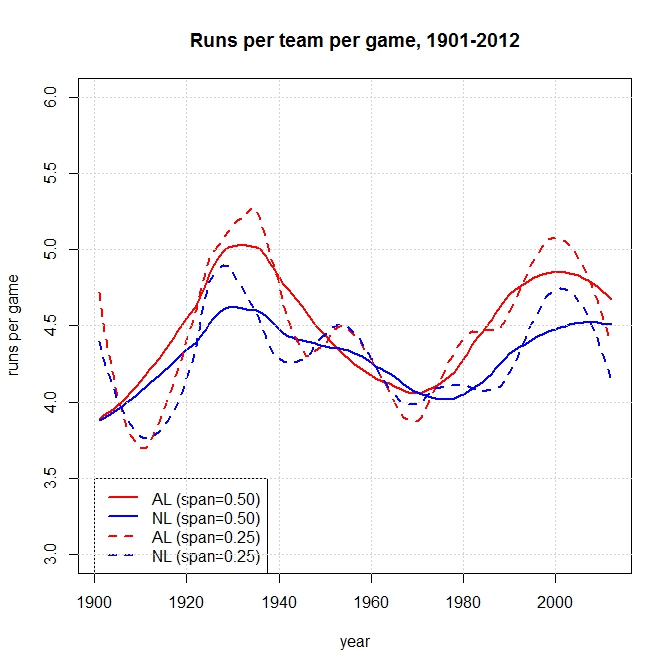
The code (available as a gist here, downloadable as an R script file) creates a pair of tables, calculating each league’s run scoring rates by year. Then, recycling my earlier code, it calculates a series of trend lines using the loess method, and graphs those trend lines. For simplicity’s sake, only the final version of each graph is shown.
Step 1: install the package (if you haven’t already), access the library, and load the data table “Teams”.
# load the package into R, and open the data table 'Teams' into the
# workspace
library("Lahman")
data(Teams)
#
The second step is to use the individual team season results to calculate the aggregate of each league’s year. We start with 1901, the year the American League was formed. Once those tables are created, the loess function is used to calculate trend lines for each league’s run scoring environment.
# ===== CREATE LEAGUE SUMMARY TABLES
#
# select a sub-set of teams from 1901 [the establishment of the American
# League] forward to 2012
Teams_sub <- as.data.frame(subset(Teams, yearID > 1900))
# calculate each team's average runs and runs allowed per game
Teams_sub$RPG <- Teams_sub$R/Teams_sub$G
Teams_sub$RAPG <- Teams_sub$RA/Teams_sub$G
# create new data frame with season totals for each league
LG_RPG <- aggregate(cbind(R, RA, G) ~ yearID + lgID, data = Teams_sub, sum)
# calculate league + season runs and runs allowed per game
LG_RPG$LG_RPG <- LG_RPG$R/LG_RPG$G
LG_RPG$LG_RAPG <- LG_RPG$RA/LG_RPG$G
# select a sub-set of teams from 1901 [the establishment of the American
# League] forward to 2012 read the data into separate league tables
ALseason <- (subset(LG_RPG, yearID > 1900 & lgID == "AL"))
NLseason <- (subset(LG_RPG, yearID > 1900 & lgID == "NL"))
#
# ===== TRENDS: RUNS SCORED PER GAME
#
# AMERICAN LEAGUE create new object ALRunScore.LO for loess model
ALRunScore.LO <- loess(ALseason$LG_RPG ~ ALseason$yearID)
ALRunScore.LO.predict <- predict(ALRunScore.LO)
# create new objects RunScore.Lo.XX for loess models with 'span' control
# span = 0.25
ALRunScore.LO.25 <- loess(ALseason$LG_RPG ~ ALseason$yearID, span = 0.25)
ALRunScore.LO.25.predict <- predict(ALRunScore.LO.25)
# span = 0.5
ALRunScore.LO.5 <- loess(ALseason$LG_RPG ~ ALseason$yearID, span = 0.5)
ALRunScore.LO.5.predict <- predict(ALRunScore.LO.5)
# NATIONAL LEAGUE create new object RunScore.LO for loess model
NLRunScore.LO <- loess(NLseason$LG_RPG ~ NLseason$yearID)
NLRunScore.LO.predict <- predict(NLRunScore.LO)
# loess models
NLRunScore.LO.25 <- loess(NLseason$LG_RPG ~ NLseason$yearID, span = 0.25)
NLRunScore.LO.25.predict <- predict(NLRunScore.LO.25)
NLRunScore.LO.5 <- loess(NLseason$LG_RPG ~ NLseason$yearID, span = 0.5)
NLRunScore.LO.5.predict <- predict(NLRunScore.LO.5)
#
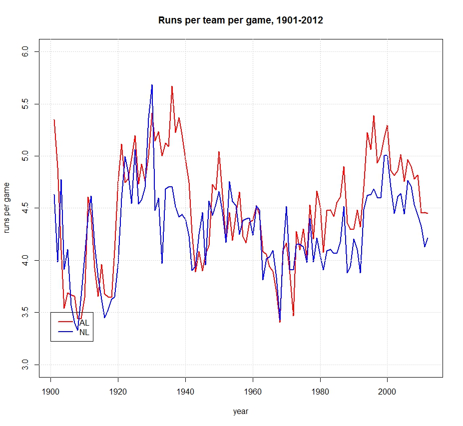
Now that we have calculated the league averages and trend lines (using the loess method), we can start the plots. First, a simple plot of the actual values:
# MULTI-PLOT -- MERGING AL AND NL RESULTS plot individual years as lines
ylim <- c(3, 6)
# start with AL line
plot(ALseason$LG_RPG ~ ALseason$yearID, type = "l", lty = "solid", col = "red",
    lwd = 2, main = "Runs per team per game, 1901-2012", ylim = ylim, xlab = "year",
    ylab = "runs per game")
# add NL line
lines(NLseason$yearID, NLseason$LG_RPG, lty = "solid", col = "blue", lwd = 2)
# chart additions
grid()
legend(1900, 3.5, c("AL", "NL"), lty = c("solid", "solid"), col = c("red", "blue"),
    lwd = c(2, 2))
# plot multiple loess curves (span=0.50 and 0.25)
ylim <- c(3, 6)
# start with AL line
plot(ALRunScore.LO.5.predict ~ ALseason$yearID, type = "l", lty = "solid", col = "red",
    lwd = 2, main = "Runs per team per game, 1901-2012", ylim = ylim, xlab = "year",
    ylab = "runs per game")
# add NL line
lines(NLseason$yearID, NLRunScore.LO.5.predict, lty = "solid", col = "blue",
    lwd = 2)
# add 0.25 lines
lines(ALseason$yearID, ALRunScore.LO.25.predict, lty = "dashed", col = "red",
    lwd = 2)
lines(NLseason$yearID, NLRunScore.LO.25.predict, lty = "dashed", col = "blue",
    lwd = 2)
# chart additions
legend(1900, 3.5, c("AL (span=0.50)", "NL (span=0.50)", "AL (span=0.25)", "NL (span=0.25)"),
    lty = c("solid", "solid", "dashed", "dashed"), col = c("red", "blue", "red",
        "blue"), lwd = c(2, 2, 2, 2))
grid()
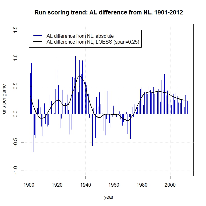
# 1. absolute
RunDiff <- (ALseason$LG_RPG - NLseason$LG_RPG)
# 2. LOESS span=0.25
RunDiffLO <- (ALRunScore.LO.25.predict - NLRunScore.LO.25.predict)
#
And plot the differences.
# plot each year absolute difference as bar, difference in trend as line
ylim <- c(-1, 1.5)
plot(RunDiff ~ ALseason$yearID, type = "h", lty = "solid", col = "blue", lwd = 2,
    main = "Run scoring trend: AL difference from NL, 1901-2012", ylim = ylim,
    xlab = "year", ylab = "runs per game")
# add RunDiff line
lines(ALseason$yearID, RunDiffLO, lty = "solid", col = "black", lwd = 2)
# add line at zero
abline(h = 0, lty = "dotdash")
# chart additions
grid()
legend(1900, 1.5, c("AL difference from NL: absolute", "AL difference from NL, LOESS (span=0.25)"),
    lty = c("solid", "solid"), col = c("blue", "black"), lwd = c(2, 2))

#
The one after that: ggplot2 versions of the graphs.
-30-
To leave a comment for the author, please follow the link and comment on their blog: Bayes Ball.
R-bloggers.com offers daily e-mail updates about R news and tutorials about learning R and many other topics. Click here if you're looking to post or find an R/data-science job.
Want to share your content on R-bloggers? click here if you have a blog, or here if you don't.