
Introducing: Orthogonal Nonlinear Least-Squares Regression in R
Want to share your content on R-bloggers? click here if you have a blog, or here if you don't.
With this post I want to introduce my newly bred ‘onls’ package which conducts Orthogonal Nonlinear Least-Squares Regression (ONLS):
http://cran.r-project.org/web/packages/onls/index.html.
Orthogonal nonlinear least squares (ONLS) is a not so frequently applied and maybe overlooked regression technique that comes into question when one encounters an “error in variables” problem. While classical nonlinear least squares (NLS) aims to minimize the sum of squared vertical residuals, ONLS minimizes the sum of squared orthogonal residuals. The method is based on finding points on the fitted line that are orthogonal to the data by minimizing for each ")

")
onls has been developed for easy future algorithm tweaking in R. The results obtained from onls are exactly similar to those found in the original implementation [1, 2]. It is based on an inner loop using optimize for each 
![[x_{i-w}, x_{i+w}]](https://s0.wp.com/latex.php?latex=%5Bx_%7Bi-w%7D%2C+x_%7Bi%2Bw%7D%5D&bg=ffffff&%23038;fg=333333&%23038;s=0 "[x_{i-w}, x_{i+w}]")
nls.lm of the ‘minpack’ package. Sensible starting parameters for onls are obtained by prior fitting with standard nls, as parameter values for ONLS are usually fairly similar to those from NLS.
There is a package vignette available with more details in the “/onls/inst” folder, especially on what to do if fitting fails or not all points are orthogonal. I will work through one example here, the famous DNase 1 dataset of the nls documentation, with 10% added error. The semantics are exactly as in nls, albeit with a (somewhat) different output:
> DNase1 <- subset(DNase, Run == 1)

> DNase1$density <- sapply(DNase1$density, function(x) rnorm(1, x, 0.1 * x))

> mod1 <- onls(density ~ Asym/(1 + exp((xmid - log(conc))/scal)),

             data = DNase1, start = list(Asym = 3, xmid = 0, scal = 1))
Obtaining starting parameters from ordinary NLS...

  Passed...

 Relative error in the sum of squares is at most `ftol'.

Optimizing orthogonal NLS...

  Passed... Relative error in the sum of squares is at most `ftol'.
The print.onls method gives, as in nls, the parameter values and the vertical residual sum-of-squares. However, the orthogonal residual sum-of-squares is also returned and MOST IMPORTANTLY, information on how many points
> print(mod1)

Nonlinear orthogonal regression model

  model: density ~ Asym/(1 + exp((xmid - log(conc))/scal))

   data: DNase1

 Asym  xmid  scal

2.422 1.568 1.099

 vertical residual sum-of-squares: 0.2282

 orthogonal residual sum-of-squares: 0.2234

 PASSED: 16 out of 16 fitted points are orthogonal.
Number of iterations to convergence: 2

Achieved convergence tolerance: 1.49e-08
Checking all points for orthogonality is accomplished using the independent checking routine check_o which calculates the angle between the slope 

onls-minimized Euclidean distance between
=> ![\alpha_i[^{\circ}] = \tan^{-1} \left( \left|\frac{\mathrm{m}_i - \mathrm{n}_i}{1 + \mathrm{m}_i \cdot \mathrm{n}_i}\right| \right) \cdot \frac{360}{2\pi}](https://s0.wp.com/latex.php?latex=%5Calpha_i%5B%5E%7B%5Ccirc%7D%5D+%3D+%5Ctan%5E%7B-1%7D+%5Cleft%28+%5Cleft%7C%5Cfrac%7B%5Cmathrm%7Bm%7D_i+-+%5Cmathrm%7Bn%7D_i%7D%7B1+%2B+%5Cmathrm%7Bm%7D_i+%5Ccdot+%5Cmathrm%7Bn%7D_i%7D%5Cright%7C+%5Cright%29+%5Ccdot+%5Cfrac%7B360%7D%7B2%5Cpi%7D&bg=ffffff&%23038;fg=333333&%23038;s=0 "\alpha_i[^{\circ}] = \tan^{-1} \left( \left|\frac{\mathrm{m}_i - \mathrm{n}_i}{1 + \mathrm{m}_i \cdot \mathrm{n}_i}\right| \right) \cdot \frac{360}{2\pi}")

 = \left|\frac{\mathrm{m}_i - \mathrm{n}_i}{1 + \mathrm{m}_i \cdot \mathrm{n}_i}\right|")
}{dx_{0i}}, \,\, \mathrm{n}_i = \frac{y_i - y_{0i}}{x_i - x_{0i}}")
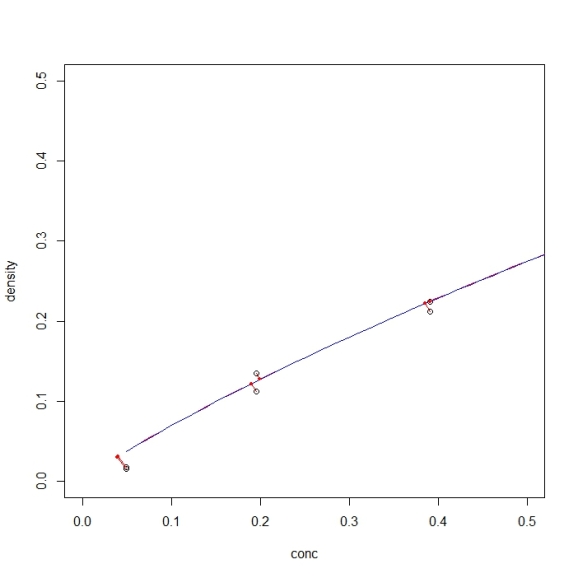
When plotting an ONLS model with the plot.onls function, it is important to know that orthogonality is only evident with equal scaling of both axes:
> plot(mod1, xlim = c(0, 0.5), ylim = c(0, 0.5))
As with nls, all generics work:
print(mod1), plot(mod1), summary(mod1), predict(mod1, newdata = data.frame(conc = 6)), logLik(mod1), deviance(mod1), formula(mod1), weights(mod1), df.residual(mod1), fitted(mod1), residuals(mod1), vcov(mod1), coef(mod1), confint(mod1).
However, deviance and residuals deliver the vertical, standard NLS values. To calculate orthogonal deviance and obtain orthogonal residuals, use deviance_o and residuals_o.
[1] ALGORITHM 676 ODRPACK: Software for Weighted Orthogonal Distance Regression.
Boggs PT, Donaldson JR, Byrd RH and Schnabel RB.
ACM Trans Math Soft (1989), 15: 348-364.
[2] User’s Reference Guide for ODRPACK Version 2.01.
Software for Weighted Orthogonal Distance Regression.
Boggs PT, Byrd RH, Rogers JE and Schnabel RB.\
NISTIR (1992), 4834: 1-113.
Cheers,
Andrej
Filed under: nonlinear regression, Uncategorized Tagged: nonlinear, ODRPACK, orthogonal, regression

R-bloggers.com offers daily e-mail updates about R news and tutorials about learning R and many other topics. Click here if you're looking to post or find an R/data-science job.
Want to share your content on R-bloggers? click here if you have a blog, or here if you don't.