
Down and Dirty Forecasting: Part 2
[This article was first published on OutLie..R, and kindly contributed to R-bloggers]. (You can report issue about the content on this page here)
Want to share your content on R-bloggers? click here if you have a blog, or here if you don't.
This is the second part of the forecasting exercise, where I am looking at a multiple regression. To keep it simple I chose the states that boarder WI and the US unemployment information for the regression. Again this is a down and dirty analysis, I would not call this complete in any sense.Want to share your content on R-bloggers? click here if you have a blog, or here if you don't.
#getting the data for WI, US, IL, MI, MN, IO
#Using Quandl data, great little site
wi<-read.csv('http://www.quandl.com/api/v1/datasets/FRED/WIUR.csv?&auth_token=gigXwpxd6Ex91cjgz1B7&trim_start=1976-01-01&trim_end=2013-04-01&sort_order=desc', colClasses=c('Date'='Date'))
us<-read.csv('http://www.quandl.com/api/v1/datasets/FRED/UNRATE.csv?&auth_token=gigXwpxd6Ex91cjgz1B7&trim_start=1976-01-01&trim_end=2013-04-01&sort_order=desc', colClasses=c('Date'='Date'))
il<-read.csv('http://www.quandl.com/api/v1/datasets/FRED/ILUR.csv?&auth_token=gigXwpxd6Ex91cjgz1B7&trim_start=1976-01-01&trim_end=2013-04-01&sort_order=desc', colClasses=c('Date'='Date'))
mi<-read.csv('http://www.quandl.com/api/v1/datasets/FRED/MIUR.csv?&auth_token=gigXwpxd6Ex91cjgz1B7&trim_start=1976-01-01&trim_end=2013-04-01&sort_order=desc', colClasses=c('Date'='Date'))
mn<-read.csv('http://www.quandl.com/api/v1/datasets/FRED/MNUR.csv?&auth_token=gigXwpxd6Ex91cjgz1B7&trim_start=1976-01-01&trim_end=2013-04-01&sort_order=desc', colClasses=c('Date'='Date'))
io<-read.csv('http://www.quandl.com/api/v1/datasets/FRED/IAUR.csv?&auth_token=gigXwpxd6Ex91cjgz1B7&trim_start=1976-01-01&trim_end=2013-04-01&sort_order=desc', colClasses=c('Date'='Date'))
#merging the data into one dataframe
#I started with WI so that I could isolate the rest of the variables better
unemp<-merge(wi, io, by='Date'); colnames(unemp)<-c('Date', 'wi', 'io')
unemp<-merge(unemp, mi, by='Date'); colnames(unemp)<-c('Date', 'wi', 'io', 'mi')
unemp<-merge(unemp, mn, by='Date'); colnames(unemp)<-c('Date', 'wi', 'io', 'mi', 'mn')
unemp<-merge(unemp, us, by='Date'); colnames(unemp)<-c('Date', 'wi', 'io', 'mi', 'mn', 'us')
unemp<-merge(unemp, il, by='Date'); colnames(unemp)<-c('Date', 'wi', 'io', 'mi', 'mn', 'us', 'il')
save(unemp, file='Unemployment WI.RData')
library(car)
library(lmtest)
library(forecast)
load('Unemployment WI.RData')
unemp.b<-unemp[1:436,]
unemp.p<-unemp[437:448,]
plot(unemp$Date, unemp$us, col='black',
main='Unemployment WI Region', type='l', xlab='Date',
ylab='Unemp. Rate', ylim=c(2, 17))
lines(unemp$Date, unemp$il, col='blue')
lines(unemp$Date, unemp$io, col='dark green')
lines(unemp$Date, unemp$mi, col='purple')
lines(unemp$Date, unemp$mn, col='gray')
lines(unemp$Date, unemp$wi, col='red')
leg.txt<-c('US', 'IL', 'IO', 'MI', 'MN', "WI")
leg.col<-c('black','blue', 'dark green', 'purple', 'gray', 'red')
legend('topleft', leg.txt, col=leg.col, pch=15)
summary(unemp)
#correlation matrix
cm<-cor(unemp[,-1])
cm
#From the graph and correlation matrix, everything
#is highly correlated, the lowest r value is 0.7879
#between Iowa and US.
#plots of each of the data, then each individual,
#everything looks really good, nice linear trends,
#although Michigan has quite bit of volatility
#compared to the other variables.
plot(unemp.b, pch='.')
model<-lm(wi~., data=unemp.b[,-1])
step.m<-step(model, direction='backward')
summary(step.m)
#testing for outliers
outlierTest(step.m)
# After conducting the outlier test, looks like it is michigan
#Sept 1980 where unemployment was 13.2 percent, point 57 is
#close at 12.9 those are the two biggest, but the outlierTest
#isolated row 56
dwtest(step.m)
dwtest(step.m, alternative='two.sided')
#yep lots of autocorrelation, so a multiple ARAIMA might be in order
pred<-unemp.p[3:7]
mult.f<-predict(step.m, newdata=pred, interval='prediction')
a1<-accuracy(mult.f, unemp.p$wi)
#because the MASE is missing I needed to add the following to compare later
a1<-c(a1,'0')
names(a1)<-c("ME", "RMSE", "MAE", "MPE", "MAPE", "MASE")
# ARIMA
auto.r<-auto.arima(unemp.b$wi, xreg=unemp.b[,3:7])
auto.r
auto.f<-forecast(auto.r, xreg=unemp.p[,3:7], h=12)
a2<-accuracy(auto.f, unemp.p$wi)
a2
#Just remember that the 0 is just a place holder
r.table<-rbind(a1, a2)
row.names(r.table)<-c('Multiple Regression', 'Reg. with ARIMA Errors')
r.table
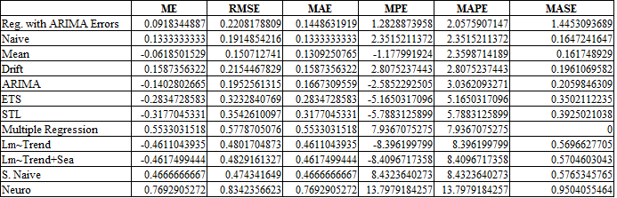
At this point I combined the two accuracy tables to see which one was the best.
b.table<-rbind(a.table[,1:6], r.table)
b.table<-b.table[order(b.table$MAPE),]
b.tableThe winner is: Regression with ARIMA Errors, for most of the analysis the simple mean like predictions dominated, even the multiple regression is considerably low on the list.
To leave a comment for the author, please follow the link and comment on their blog: OutLie..R.
R-bloggers.com offers daily e-mail updates about R news and tutorials about learning R and many other topics. Click here if you're looking to post or find an R/data-science job.
Want to share your content on R-bloggers? click here if you have a blog, or here if you don't.