Gradient descent is a fundamental concept in machine learning, and therefore one practitioners should be familiar with. In this post we will explore gradient descent from both theoretical and practical perspectives. First, we will establish some general definitions, review cost functions in the context of regression and binary classification, and introduce the chain rule of calculus. Then, we will put it all into practice to build a linear and a logistic regression models from the ground up. This is a short, introductory guide where a basic knowledge of statistics and calculus should be most helpful. Ready, set, go!

Introduction

Most predictive algorithms learn by estimating a set of parameters – also known as weights, or coefficients – that minimise the cost function, a measure of prediction error. In gradient-based learning, that search process invariably employs gradient descent or one of its numerous extensions. Gradients are partial derivatives of the cost function with respect to each model parameter, . On a high level, gradient descent is an iterative procedure that computes predictions and updates parameter estimates by subtracting their corresponding gradients weighted by a learning rate . This procedure will find estimates that incur ever smaller prediction errors, provided i) the learning rate is adequate, ii) the maximum number of iterations is sufficient and iii) the underlying dataset is suitable for modelling.

How gradient descent works will become clearer once we establish a general problem definition, review cost functions and derive gradient expressions using the chain rule of calculus, for both linear and logistic regression.

Problem definition

We start by establishing a general, formal definition. Suppose we have a matrix carrying p predictors observed across n observations, and the vector of parameters comprising the model intercept and the slopes from each individual predictor. Our aim is to predict some target y using a combination of  and :

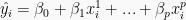
• In linear regression, we would like to predict the continuous target variable . The model prediction from any observation i takes the form
• In logistic regression, we would like to predict the binary target variable . The model prediction from any observation i takes the form , where is the logit of y, and is the logistic function that transforms logit to target probability

Note that in linear and logistic regression, in one shot you can directly access all n predictions and logit values, respectively, via the matrix product after appending a column of ones to the left of .

Cost function

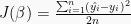
In both linear and logistic regression, the aim is to find the parameter estimates that minimise the prediction error. This error is generally measured using a cost function:

• In linear regression, one can use the mean squared error (MSE), . It measures the average squared difference between the observed and predicted target values (lower is better)
• In logistic regression, one can use the binary cross-entropy, . It measures the amount of uncertainty shared between the observed and estimated probability distributions (lower is better)

Putting it together, we have a recipe to predict a target using  and , and measure the error between resulting prediction and the target. What are we missing then?

Gradient descent

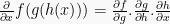
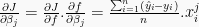
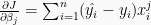
As we saw earlier, gradient descent is mainly driven by the partial derivatives of the cost function with respect to each individual parameter, . So, how do we calculate these?

To this end, we can use of the chain rule of calculus, which posits that  for any number of functions, to simplify the derivative of a cost function with respect to any parameter. Assuming , which turns out to be and the logit  for linear and logistic regressions respectively, we find that:

• For linear regression using a MSE cost function , we can decompose the derivative of the cost function into two parts, 
• For logistic regression using a binary cross-entropy cost function , we can decompose the derivative of the cost function into three parts,  , or equivalently 

In both cases the application of gradient descent will iteratively update the parameter vector  using the aforementioned equation . Also, it is worth noting that none of the predictors contributes to the intercept partial derivative, i.e. .

Now, I encourage you to apply the chain rule and try deriving these gradient expressions by hand, using the provided definitions of , and accordingly

Let’s get started with R

Let us now apply these learnings to build two models using R:

• Linear regression, to predict the age of orange trees from their circumference
• Logistic regression, to predict engine shape from miles-per-gallon (mpg) and horsepower

In both cases we will implement batch gradient descent, where all training observations are used in each iteration. Mini-batch and stochastic gradient descent are popular alternatives that use instead a random subset or a single training observation, respectively, making them computationally more efficient when handling large sample sizes. Make sure that you have RColorBrewer installed.

Linear regression

Our first model, based on the Orange dataset, will have the following structure:

In the code below we will configure gradient descent such that in each of 25 iterations, a prediction is made and the two parameters and are updated using the gradient expressions presented earlier, using the learning rate . We will also designate the two parameters as b0 and b1, then plot and store their estimates under the lists intercepts and slopes, respectively. Finally, we will create a MSE cost function contour to visualise the trajectory of the same parameter estimates in the course of gradient descent.

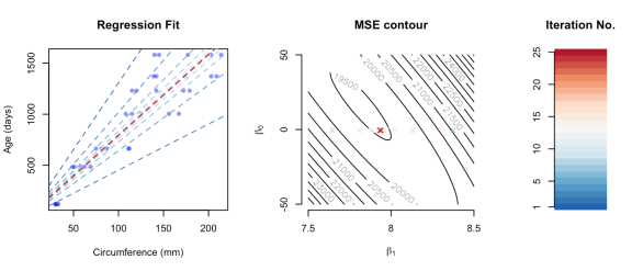
By colouring the iterations from blue (early) to red (late) using a diverging palette, we can see how gradient descent arrived at parameter estimates that minimise the prediction error! In addition, the contour suggests that an optimal regression fit can be obtained using a small-intercept, large-coefficient combination or vice versa. Finally, note that the variation in the values of in the right-hand panel is concealed by the scale used in the MSE contour plot, intentionally set for ease of contour visualisation.

Logistic regression

Our second model, based on the mtcars dataset, will have the following structure:

which is reminiscent of the generalised linear model employed in the past introduction to Bayesian models. In the code below, we will configure gradient descent such that in each of 100 iterations, a prediction is made and the three parameters , and  are updated using the gradient expressions presented earlier, using the learning rate . We will also designate the three parameters as b0,  b1 and b2 and store their estimates under the lists intercepts, slopes1 and slopes2,  respectively. Lastly, we will calculate and visualise the decision boundary from each iteration and examine how the parameter estimates change in the process.

CALCULATING THE DECISION BOUNDARY

The decision boundary can be determined from setting the logit expression to zero – equivalent to a target probability of 50% – then solving for either mpg or horsepower:

Solving for mpg here, we only need to pick at least two arbitrary values of horsepower, find their corresponding mpg values and connect the points with a line, in each iteration

Applying the same colouring scheme, we can see how gradient descent arrived at parameter estimates that minimise the prediction error! Note how the decision boundary neatly separates most members of the two engine shape classes. In addition, the right-hand panel shows how the slope parameters and change steadily, at different rates until they plateau, while the intercept is readily defined early on.

Conclusion

Well done, we have just learned and applied gradient descent! Time to recap all the steps taken:

• A general problem definition was set to assign predictors, target, parameters and learning rate to well defined mathematical entities
• The MSE and the binary cross-entropy cost functions were introduced
• The chain rule of calculus was presented and applied to arrive at the gradient expressions based on linear and logistic regression with MSE and binary cross-entropy cost functions, respectively
• For demonstration, two basic modelling problems were solved in R using custom-built linear and logistic regression, each based on the corresponding gradient expressions

Finally, here are some ideas of where to go from here:

• Customisation. One major advantage of knowing the nuts and bolts of gradient descent is the high degree of customisation it allows. You could, for example, use the above recipe to add parameter regularisation to a cost function and derive the updated gradient expressions
• Interpretation. Although the focus of our two exercises was computational, I urge you to make sense of the resulting parameter estimates. It seems obvious that older trees have wider circumferences, not so much that V-shaped engines provide less mpg. Can we create models that explore causality? How much does a unit change in each predictor impact the target prediction? To me, these sort of questions serve as an enjoyable sanity check
• Experimentation. Use the code above as a template to experiment with different learning rates and number of iterations. Recall that the learning rate determines the step size of each parameter update, while the number of iterations determines how long learning takes place. Do your experiments conform to expected results?
• Benchmarking. It could be interesting to compare our estimation results with those obtained from using lm()  and glm()  or similar. Do parameter estimates agree between? Which algorithm is faster? How do they differ?  

I hope this tutorial has rekindled your interest in machine learning, inspired novel applications and demystified the underlying mathematics. As usual, please enter a comment below – a question, a suggestion, praise or criticism. Until next time!

Citation

de Abreu e Lima, F (2023). poissonisfish: Gradient descent in R. From https://poissonisfish.com/2023/04/11/gradient-descent/