Chapter 5: Part 1, Real Markets

This is the supplement to Chapter 5 of my book, Goals-Based Portfolio Theory, demonstrating the techniques and offering some code examples. If you are reading this having not purchased/read the book, you are missing much of the narrative. You can pick up a copy from Wiley, Amazon.com, or Barnes & Noble.

Are Markets Tractors… Or Horses?

Growing up on a cattle ranch in central Texas, I developed a certain respect for the tools of the trade. Horses, tractors, trucks, trailers, bailing wire, and duct tape were all daily-use items for us.

Each tool has its purpose, of course, and each tool has advantages and disadvantages for a particular job. Take, for example, the contrast between horses and tractors.

As you might well imagine, you can get quite a lot done with a tractor. You can plow a field, fix fences, haul hay. But the best thing about a tractor is that you can get up every morning and turn it on, do your work, come home, and turn it off. So long as it has fuel, it will do what you tell it to do.

You can also get a lot done with a horse. Horses have different advantages, like getting to those hard-to-reach places on your land. Their agility makes them particularly good at herding other animals. But horses are bigger and stronger than we are and unlike tractors, they have a mind of their own. If you wake up to a horse who has decided she isn’t going to work today, there really isn’t much you can do about it!

One of the biggest mistakes I see investors make — especially professional investors — is to treat financial markets like tractors. They expect to wake up every day to a reliable and consistent tool that helps them achieve their financial goals. “So long as we keep this tractor well-oiled, maintained, and full of diesel,” the thinking goes, “it’ll keep moving us closer to our goal.”

But in my experience, financial markets are much more like horses. They have a mind of their own and they are bigger and stronger than we are! Sure you can get a lot done with markets, but there are some days they would just as soon buck you off as get your work done. (from “On Horses, Tractors, and Markets”, Enterprising Investor)

In Chapter 5 of my book, I point out that stock markets are, most likely, Levy alpha-stable distributions (bitcoin almost certainly is, but more on that in a different post). Let’s use R to generate the two examples I use there.

Example 1: N-Day Volatility

The first example I look at is N-day volatility of the S&P 500. If SPX had a Gaussian distribution, then taking the first 1000 days of volatility should be more than enough data to infer the next 1000 days of volatility. As it turns out, this is not the case! (This is an idea that I pulled from Fractal Market Analysis by Edgar Peters).

Let’s begin by loading libraries:

library(quantmod)
library(tidyverse)
library(libstableR)

Then, let’s pull daily S&P 500 data from Yahoo!Finance and clean the data to use only dividend-adjusted figures:

getSymbols( '^GSPC', from = '1970-01-01', to = '2020-01-01' )
spy <- GSPC$GSPC.Adjusted %>% Delt(k=1) %>% na.omit()

Now, we are going to measure the volatility of prices for 2 days, then 3 days, then 4 days, and so on, up to 12,612 days (hence “N-day”). I do this using a for-loop, but there may be a more “R way” to do it.

n_day_s <- 0
n <- 0
for(i in 1:length(spy)){
  n_day_s[i] <- sd( coredata(spy[1:i]) )
  n[i] <- length(spy[1:i])
}

Next, let’s look at the volatility for the S&P 500 for the first 1000 days of the sample. This involves taking the standard deviation of the sample, then drawing N random numbers from a Gaussian distribution that matches the parameters of the sample.

We then align the actual volatility of the S&P 500 with the expected volatility of the Gaussian distribution over each N period. Again, using a for-loop, we get:

test <- rnorm( length(spy),
               mean = mean(spy[1:1000]),
               sd = sd( spy[1:1000] ))
n_day_s_test <- 0
n <- 0
for(i in 1:length(test)){
  n_day_s_test[i] <- sd( test[1:i] )
  n[i] <- length( test[1:i] )
}

Then, we can visualize the results:

data.frame( 'Days' = c(n, n),
            'NDayVol' = c(n_day_s,
                          n_day_s_test ),
            'Label' = c( rep('Actual S&P 500', length(n)),
                         rep('Gaussian Expectation', length(n))) )%>% 
              ggplot( ., aes(x = Days, y = NDayVol, lty = Label ) )+
              geom_line( size = 1.25 )+
              xlab('Days Used to Calculate Volatility')+
              ylab('Daily Volatility')+
              theme_minimal()+
              theme( axis.title = element_text(size = 16, face = 'bold'),
                     axis.text = element_text( size = 14 ),
                     legend.title = element_blank(),
                     legend.text = element_text( size = 16, face = 'bold'),
                     legend.position = 'top')

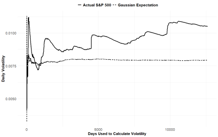
As this chart shows, the volatility of equities never actually stabilizes on one value, as we would expect from a Gaussian distribution. It is characterized by large jumps and skips that overwhelm all previous values of volatility that preceded it. If you think of these big jumps as “catastrophies” and “unexpected” you would be shocked and surprised by the next one. But, as this clearly shows, there is always a next one! It is the norm, not the outlier!

Markets really are much more like a bucking horse than a easy-going tractor.

Example 2: What if You Knew the Future?

Understanding the distribution that is at work is much more than just an academic exercise, it has dramatic real world consequences!

Suppose you have a portfolio with 60% allocated to SPY, 30% to AGG, and 10% to GLD, and sitting in 2004, you had perfect foreknowledge of the parameters of the distribution you chose to model this portfolio. Not of the returns themselves, but perfect knowledge of the parameters.

Using a Gaussian distribution assumption would actually cause you to underestimate the probability of achieving a 7% return by about 13 percentage points! Using an alpha-stable distribution as your assumption, you would be off by a mere 2 percentage points from the actual realized probability.

We can illustrate this, by pulling the returns of SPY, AGG, and GLD, then cleaning the data so we have yearly figures. Finally, the returns of the portfolio with 60% SPY, 30% AGG, and 10% GLD.

getSymbols( c('SPY', 'AGG', 'GLD') , from = '2003-01-01', to = '2020-12-
31')
spy <- to.yearly(SPY)[,6] %>% Delt(k=1) %>% na.omit()
agg <- to.yearly(AGG)[,6] %>% Delt(k=1) %>% na.omit()
gld <- to.yearly(GLD)[,6] %>% Delt(k=1) %>% na.omit()
return <- 0.60 * spy + 0.30 * agg + 0.10 * gld

Using the libstableR package, we can assess the parameters of the portfolio return distribution, both as stable-alpha and also as Gaussian:

pars_stable <- stable_fit_init( coredata(return) )
pars_stable <- stable_fit_koutrouvelis( coredata(return), pars_init = pars_stable )
pars_gauss <- c( mean(return), sd(return) )

Then we can build a simulation of both distributions and compare it to the actual distribution (note that this uses CDFs not PDFs, for the sake of the visualization).

x <- seq( -0.50, 0.50, 0.001)
stableCDF <- stable_cdf( x, pars = pars_stable )
gaussCDF <- pnorm( x, pars_gauss[1], pars_gauss[2] )
actualCDF <- 0
for(i in 1:length(x)){
  actualCDF[i] <- length( which( return <= x[i] ) ) / length(return)
}

And, finally, the visualization.

data.frame( 'Return' = c(x,
                         x,
                         x),
            'CDF' = c(stableCDF,
                      gaussCDF,
                      actualCDF),
            'Dist' = c( rep('Alpha-Stable', length(x)),
                        rep('Gaussian', length(x) ),
                        rep('Actual', length(x) ) ) ) %>% 
  ggplot(., aes(x = Return, y = CDF, lty = Dist) )+
  geom_line( size = 1.00 )+
  scale_linetype_manual( values = c('solid', 'dotted', 'dashed') )+
  xlim(-0.50, 0.50)+
  # ylim(0, 0.25)+
  xlab('Annual Return')+
  ylab('Cumulative Probability')+
  theme_minimal()+
  theme( axis.title = element_text(size = 16, face = 'bold'),
         axis.text = element_text( size = 14 ),
         legend.title = element_blank(),
         legend.text = element_text( size = 16, face = 'bold'),
         legend.position = 'top')

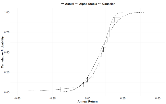
Again, we can see that the alpha stable distribution more closely describes the actual distribution of returns realized by the portfolio. The Gaussian distribution significantly underestimates the tails, and puts more expectation in the middle, which is not accurate in real life.

This has big implications for portfolio construction, especially for goals-based investors. Carrying the right distribution assumption is very important!

The next post will continue the discussion from Chapter 5, but will look at risk management through a goals-based lens.