Introduction

Natural Language Processing (NLP) is a powerful tool in the Machine Learning landscape that can (among other things) allow users to classify sentiment and predict text. Many of recent my blogs have been about data manipulation and data engineering, so I decided change things up to look into showing some applications of machine learning. In this short blog I show an application of using “Long Short Term Memory” (LSTM) networks to predict sentiment of tweets with keras in R.

The data I am going to use is the stock market sentiment dataset from Kaggle. The small (5791 row) pre-labeled dataset was contributed by Yash Chaudhary and has raw text on tweets relating to stock market news from multiple Twitter handles and their sentiment (-1 = negative, 1= positive). For construction of the model I was inspired by Tensorflow’s “Natural Language Processing (NLP) Zero to Hero” series, mselimozen’s Kaggle notebook and finnstats’ blog on LSTM networks in R.

As far as hyperparameters are concerned, the choices you see here is based is from some Googling and some trial and error. If you see anything I’m doing wrong or could do better please let me know!

Preprocessing

As far as processing is concerned, the use of setting a seed for reproducibility and re-coding sentiment to be binary with negative sentiment being re-coded as 0 was done. A 75%-25% training-testing split was done on the dataset as well. After tokenizing the training set of data, the datasets were sequenced and padded. The code to do this is adapted from the “Zero to Hero” series. The data prep essentially follows the content there but is slightly altered by according to what I’ve seen other folks do.

set.seed(4289)
library(keras)
library(tidyverse)

# Reading Data, re-coding sentiment. 
stock_tweets <- readr::read_csv("stock_data.csv") %>% 
                mutate(Sentiment = ifelse(Sentiment==-1,0,1))

# 75%-25% Training-Testing Split
smp_size <- floor(0.75 * nrow(stock_tweets))

train_ind <- sample(seq_len(nrow(stock_tweets)), size = smp_size)

train <- stock_tweets[train_ind, ]
test <- stock_tweets[-train_ind, ]

vocab_size<-10000

# Tokenizer
tokenizer <- text_tokenizer(num_words=vocab_size,
                            oov_token = "<OOV>")
tokenizer$fit_on_texts(texts=train$Text)
# Word Index
word_index <- tokenizer$word_index
# Sequencing.
training_sequences <- tokenizer$texts_to_sequences(train$Text)
testing_sequences <- tokenizer$texts_to_sequences(test$Text)

# Padding 
training_padded <- pad_sequences(training_sequences,
                                 maxlen = 128,
                                 padding='post',
                                 truncating = 'post')
testing_padded <- pad_sequences(testing_sequences,
                                maxlen = 128,
                                padding='post',
                                truncating = 'post')

Modelling

The layers for this model were chosen through messing around. I wish I had a more technical term to describe it. Using a binary cross-entropy loss function and a Adam optimizer were great for improving accuracy. I’m sure there’s a way to get better accuracy but I’m impressed with getting over 70% validation accuracy the model produced with such a small dataset.

After playing around with this for a bit, I think the primary method to improve accuracy would be to get more data and retrain the model. If you know of a larger dataset that is similar to this, please let me know to see if my theory is correct!

set.seed(4289)
embedding_dim <- 128

model <- keras_model_sequential() %>% 
         layer_embedding(vocab_size,
                         embedding_dim,
                         input_length=128) %>%
          layer_lstm(units = 128,return_sequences = TRUE) %>% 
          layer_lstm(units = 64,return_sequences = TRUE) %>% 
          layer_lstm(units = 32,return_sequences = TRUE) %>%
          layer_lstm(units = 16,return_sequences = TRUE) %>%
          bidirectional(layer_lstm(units =8)) %>%
          layer_dense(8,activation = "sigmoid") %>%
          layer_dense(1,activation = "sigmoid")  
model$compile(loss='binary_crossentropy',optimizer="adam",metrics=c('accuracy'))

history<-fit(model, 
    x = training_padded, 
    y = train$Sentiment, 
    epochs = 10,
    verbose = getOption("keras.fit_verbose", default = 1),
    validation_split = 0.3, 
    validation_data = list(testing_padded,test$Sentiment))

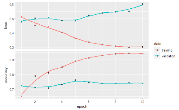
history


## 
## Final epoch (plot to see history):
##         loss: 0.2059
##     accuracy: 0.9415
##     val_loss: 0.8044
## val_accuracy: 0.7396


plot(history)

evaluate(model,x=testing_padded,y=test$Sentiment)


##      loss  accuracy 
## 0.8043559 0.7396409

Conclusion

As mentioned before, the deep learning model developed here was inspired from other tutorials. When I was taking machine learning in university, I was told that the choice of layers and hyper parameters is “an art”. Is this true or is there more of a methodical approach to building predictive models with deep learning? Please let me know or point me to your favorite resources!

Thank you for reading!