Building a Model in R to Predict FPL Points

Fantasy premier league. That yearly ritual of thinking your team you spend hours agonising over whether to select this player or that player. I find you need to watch a lot of football to keep up with it so the challenge is how can I use data to shortcut this. This is probably the biggest challenge I have taken up in R so lets see how I get on.

Building the model its important to have a clear state of the aim and that for this is clearly an estimation of the points a player might achieve in a game week or over several game weeks. First things first I need data and most of that data is conveniently available in the fplsrapr package. The get_player_details function from the package prints a table with the required seasons stats. To create this plot I did that for all seasons and that created one data frame of all the data.

{r}
season18 <- get_player_details(season = 18) # the function used to download the match by match data for each player from the fpl scrapr package. The season argument is the season 18/19 


# taking each seasons data filtering the required columns and then putting them all together
s16p <- season16 %>% filter(minutes > 0) %>%
                            select(playername, total_points, fixture)


s17p <- season17 %>% filter(minutes > 0) %>%
                            select(playername, total_points, fixture)


s19p <- season19 %>% filter(minutes > 0) %>%
                            select(playername, total_points, fixture)

# creating the dataframe for total  points
totpo <- s16p %>% 
                  bind_rows(s17p) %>%
                    bind_rows(s18p) %>%
                      bind_rows(s19p)

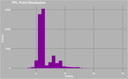
If you have a normally distributed target variable then it makes it much easier to model. This though is not even close to any distribution and I think that’s because of the randomness of football and there’s a certain type of player that are much more successful. Also the point system used in the game means there’s no an equal chance of all numbers appearing. Using the same data set I created the comparison between 2 players in the same team

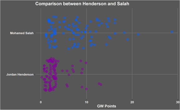
The graph above shows the point of the model. They are both players who play in midfield for the same team therefore should have the same opportunity to score points. However, as you can see Salah scores higher points much more frequently then Henderson and therefore the model has to have information to make those determinations.

I use the dataframe I already downloaded to look at how the amount of goals scored by the teams effects how many points a player gets.

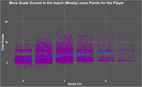
There’s not a perfect trend as you would expect. A lot of variability exists in this data due to different playing positions. There is a weak trend that total game week points increases as the amount of goals there team scores increases. There are is a clear split in a lot of the data. When there team has score no goals but lots of points scored these are mostly defenders or goalkeepers keeping clean sheets and saving penalties. When more goals are scored that’s when the strikers and attacking midfielders start to score the big points.

### collecting each players key statistics from  each season 

playdat1 <- twenty16 %>% bind_rows(twenty17) %>%
                            bind_rows(twenty18) %>%
                              bind_rows(twenty19) %>%
                                group_by(player_name) %>%
                                summarise(ninet = sum(time)/90, xgs = sum(xG), xas = sum(xA), npxGs = sum(npxG)) %>%
                                    mutate(xg90 = xgs/ninet, xA90= xas/ninet, npxg90 = npxGs / ninet) %>%
                                    select(player_name, xg90, xA90, npxg90) %>%
                                      left_join(play2, by = "player_name") %>%
                                        select(player_name, xg90, xA90, npxg90, NameID, Pos, FPLPos)




### getting each players points per 90 and then joining to the key stats ofe the player, 




playpoints <- season19 %>% group_by(playername) %>%
                              summarise(tp = sum(total_points), tm = sum(minutes)) %>%
                                mutate(p90 = tp/(tm/90)) %>%
                                    filter(tm > 270) %>%
                                    left_join(play2, by = "playername") %>%
                                      left_join(playdat1, by = "player_name") %>%
                                          filter(!is.na(FPLPos.y))


 ## creating the plot 


cols <- c("Defender" = "#8900a1", "GK" = "#c46900", "Midfielder" = "#0ea300", "Striker" = "#0042a6")

ggplot(playpoints, aes(x = xg90, y = p90, col = FPLPos.y)) + 
                                  geom_point(alpha = 0.6, size = 3) +
                                guides(colour = guide_legend(title = "Position")) +
                                        scale_colour_manual(values = cols) + labs(x = "xG/90", y = "Points/90", title = "FPL Points compared to players Expected Goals") +
  theme(panel.background = element_rect(fill = "#b8b8b8"), panel.grid.minor  = element_blank(),panel.grid.major = element_line(colour = "#363636"),  legend.background = element_rect(fill = "#b8b8b8"), plot.background = element_rect(fill = "#b8b8b8"))

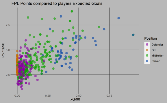
When the xG per 90 is compared to a players points per 90 you can see it has strong correlation for the points a striker will score per 90 minutes they play. It also seems to have some impact on midfielders but not impact really on defenders and goalkeepers. Therefore its good to have a source of expected goal data to make the points prediction more accurate. Goalkeepers and defenders score will mainly be impacted by by how good the opposition is so as well individual player xG90 I will be using the whole team number as well.

The key takeaway is the model needs to take into account the expected result. Then it needs to have a method to split out the attacking players from the other other players. Your Mo Salahs from your Jordan Hendersons. Therefore this model is going to be multiple separate models to make one overall model. I’m the next blog ill go through the first part of it what data I am using and where it comes from and getting the data ready for the model.