Plots within plots with ggplot2 and ggmap

Once in a while, you might find yourself wanting to embed one plot within another plot. ggplot2 makes this really easy with the annotation_custom function. The following example illustrates how you can achieve this. (For all the code in one R file, click here.)

Let’s generate some random data and make a scatterplot along with a smoothed estimate of the relationship:

library(ggplot2)

set.seed(42)
n <- 1000
x <- runif(n) * 3
y <- x * sin(1/x) + rnorm(n) / 25
df <- data.frame(x = x, y = y)

p1 <- ggplot(df, aes(x, y)) +
    geom_point(alpha = 0.3) +
    geom_smooth(se = FALSE) +
    theme_bw()
p1

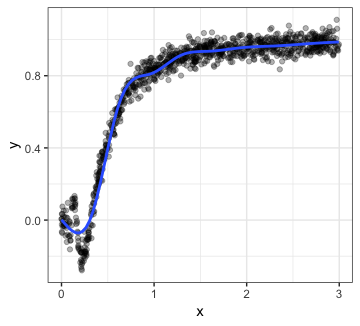
The smoother seems to be doing a good job of capturing the relationship for most of the plot, but it looks like there’s something more going on in the region. Let’s zoom in:

p2 <- ggplot(df, aes(x, y)) +
    geom_point(alpha = 0.3) +
    geom_smooth(se = FALSE) +
    scale_x_continuous(limits = c(0, 0.5)) +
    scale_y_continuous(limits = c(-0.3, 0.6)) +
    theme_bw()
p2

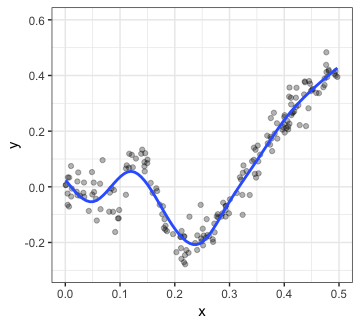
That certainly seems like a meaningful relationship! While we might want to plot p1 to depict the overall relationship, it is probably a good idea to show p2 as well. This can be achieved very easily:

p1 + annotation_custom(ggplotGrob(p2), xmin = 1, xmax = 3, 
                       ymin = -0.3, ymax = 0.6)

The first argument is for annotation_custom must be a “grob” (what is a grob? see details here) which we can create using the ggplotGrob function. The 4 other arguments (xmin etc.) indicate the coordinate limits for the inset: these coordinates are with reference to the axes of the outer plot. As explained in the documentation, the inset will try to fill up the space indicated by these 4 arguments while being center-justified.

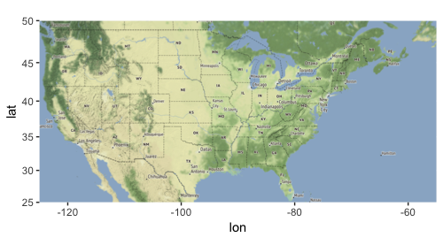
For ggmap objects, we need to use inset instead of annotation_custom. We illustrate this by making a map of continental USA with insets for Alaska and Hawaii.

Let’s get a map of continental US (for more details on how to use Stamen maps, see my post here):

library(ggmap)

us_bbox <- c(left = -125, bottom = 25, right = -55, top = 50)
us_main_map <- get_stamenmap(us_bbox, zoom = 5, maptype = "terrain")
p_main <- ggmap(us_main_map)
p_main

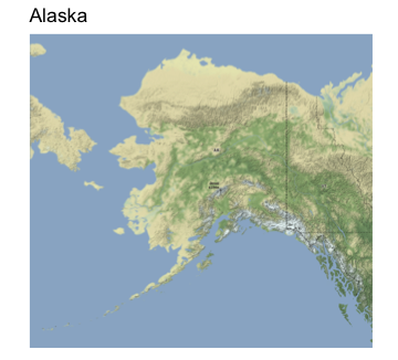
Next, let’s get maps for Alaska and Hawaii and save them into R variables. Each plot will have a title for the state, and information on the axes will be removed.

alaska_bbox <- c(left = -180, bottom = 50, right = -128, top = 72)
alaska_map <- get_stamenmap(alaska_bbox, zoom = 5, maptype = "terrain") 
p_alaska <- ggmap(alaska_map) + 
    labs(title = "Alaska") +
    theme(axis.title = element_blank(), 
          axis.text  = element_blank(),
          axis.ticks = element_blank())
p_alaska

hawaii_bbox <- c(left = -160, bottom = 18.5, right = -154.5, top = 22.5)
hawaii_map <- get_stamenmap(hawaii_bbox, zoom = 6, maptype = "terrain") 
p_hawaii <- ggmap(hawaii_map) + 
    labs(title = "Hawaii") +
    theme(axis.title = element_blank(), 
          axis.text  = element_blank(),
          axis.ticks = element_blank())
p_hawaii

We can then use inset twice to embed these two plots (I had to fiddle around with the xmin etc. options to get it to come out right):

library(grid)
p_main +
    inset(ggplotGrob(p_alaska), xmin = -76.7, xmax = -66.7, ymin = 26, ymax = 35) +
    inset(ggplotGrob(p_hawaii), xmin = -66.5, xmax = -55.5, ymin = 26, ymax = 35)