

Want to share your content on R-bloggers? click here if you have a blog, or here if you don't.
The Professional Footballers’ Association (PFA) Team of the Year is released in England at the end of each season, picking the 11 most influential players in each of Britain’s leagues.
The Team of the Year award was launched in the 1973-1974 season, meaning there was 44 years worth of data to web scrape. Using Wikipedia’s PFA Team of the Year pages (filtered by decade) and the rvest package, I was left with a dataframe of 484 soccer players (44 years * 11 players per/year).
Here are some visualizations I thought were cool:
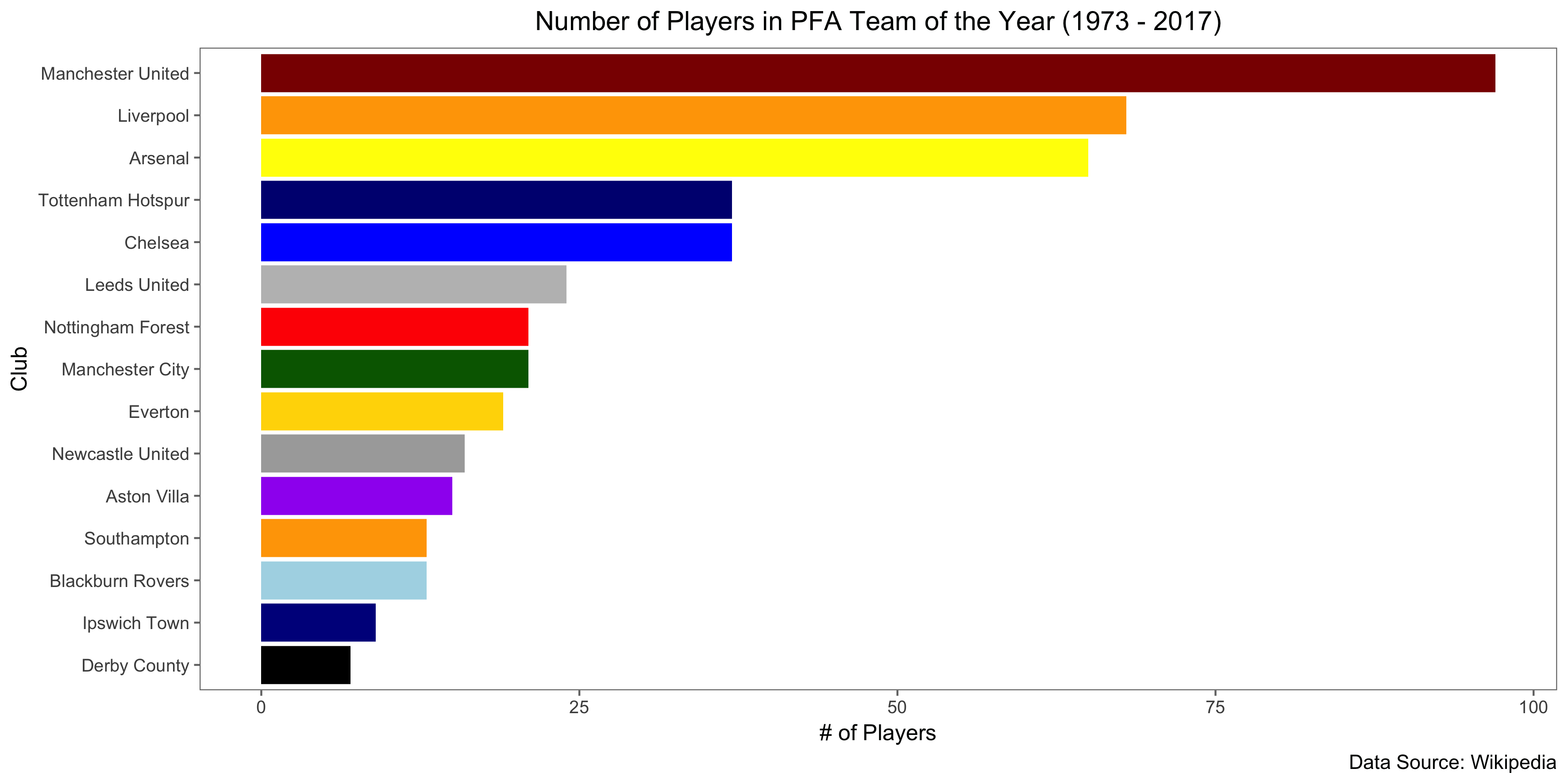
- Liverpool, Arsenal, and (most significantly) Manchester United are represented more than other clubs. United need just three more players to hit the 100 mark.
- The PFA Team of the Year formation has changed over time from 4-3-3 to 4-4-2. The graph below shows the number of forwards and midfielders who featured in the ranking each year. Up until the late 1980s, the formation included three midfielders and three forwards (the Team of the Year has always had four defenders and one goalkeeper). In the 1990s, both formations were used but since the 2000s, the use of two strikers has been the status quo.


- Additionally, I thought it was interesting to see the top individual players in each position. Peter Shilton remains the only player to hit 10 First Division PFA Team of the Year Awards.

- The more interesting analysis involved merging Team of the Year data with historical league position. We can now ask questions along the lines of: did the majority of players in the Team of the Year come from the champions that year or other teams? Looking at the specific seasons with the most representation in the award, only 14 times did a team have 5+ players on the list; the majority of these teams came from the champions (12 out of 14); only Manchester United in 1998 and Arsenal in 2003 (both runner-ups) feature in this list.

- And here are the champions of England with the fewest players on the Team of the Year. There are many from the 1970s and 1980s, which hints to a change in the way the Team of the Year was designed over the years (it may have been purposefully less top-heavy in the past, whereas today the English champions often features more significantly on the list). We can see that more recently Manchester City in 2014 and Chelsea in 2010 were on the lower end in terms of representation.

- While we’re at it, which teams that didn’t finish 1st had the most players represented? It’s clear that there were some pretty high quality teams that didn’t win the league these years (runners-up are in red, third place teams in green, and any from 4th to 20th in grey).

I think that’s enough visualizations for today, but there’s definitely a lot more we can analyze with this data. Let me know if you have any questions or feedback.
R Code Snapshot (full code can be found on Github):
Step 1 – Web Scraping:
#initialize data.frame
df <- data.frame(`Pos.`= as.character(),
Player = as.character(),
Club = as.character(),
`App.` = as.double(),
year = as.character())

div_table_numbers <- c(1,5,9,13,17,21,25,29,33,37)

urls <- c("https://en.wikipedia.org/wiki/PFA_Team_of_the_Year_(2000s)",
"https://en.wikipedia.org/wiki/PFA_Team_of_the_Year_(1990s)",
"https://en.wikipedia.org/wiki/PFA_Team_of_the_Year_(1980s)")


for (i in 1:length(urls)){

  for (j in 1:length(div_table_numbers)) {
    xpath_base <- '//*[@id="mw-content-text"]/div/table['
    new_data <- urls[i] %>%
      html() %>%
      html_nodes(xpath = paste0(xpath_base,
                              div_table_numbers[j],
                              "]")) %>%
      html_table()

     new_data <- new_data[[1]]

     year_xpath_base <- '//*[@id="mw-content-text"]/div/h3['
     year <- urls[i] %>%
      html() %>%
      html_nodes(xpath = paste0(year_xpath_base,
                              j,
                              "]")) %>%
      html_text()

      year <- year %>% str_remove_all(fixed("[edit]"))

    new_data$year <- year

    df <- bind_rows(df,
                    new_data)
  }
}
Step 2: Exploratory data analysis and visualizations
club_count <- df %>% count(Club, sort = TRUE)

club_count %>%
  top_n(n = 15) %>%
  ggplot(aes(x = reorder(Club,n),
                  y = n,
                  fill = Club)) +
  geom_col() +
  coord_flip()+
  theme_few()+
  guides(fill=FALSE)+
  labs(y = "# of Players",
       x = "Club",
       title = "Number of Players in PFA Team of the Year (1973 - 2017)",
       caption = "Data Source: Wikipedia")+
  theme(plot.title = element_text(hjust = 0.5)) +
   scale_fill_manual(values = c("Manchester United" = "darkred",
                                 "Liverpool" = "orange",
                                 "Arsenal" = "yellow",
                                 "Chelsea" = "blue",
                                 "Blackburn Rovers" = "lightblue",
                                 "Leeds United" = "grey",
                                 "Manchester City" = "dark green",
                               "Derby County" = "black",
                               "Everton" = "gold",
                               "Nottingham Forest" = "red",
                               "Ipswich Town" = "darkblue",
                               "Southampton" = "orange",
                               "Newcastle United" = "darkgrey",
                               "Aston Villa" = "purple",
                               "Tottenham Hotspur" = "navy"
                               ))
df <- df %>%
  mutate(short_year = str_sub(year,1,4) %>%
           as.numeric() + 1)

order_positions <- c("GK","DF","MF","FW")

df <- df %>% mutate(Pos. = fct_relevel(Pos., order_positions))

count_position <- df %>%
  filter(Pos. %in% c("MF","FW")) %>%
    count(Pos.,short_year, sort = TRUE)

count_position %>%
  ggplot(aes(x=short_year,y=n,color=Pos.,group=Pos.)) +
  geom_point(position=position_jitter(h=0.005))+
  geom_smooth(method = "loess")+
  scale_x_continuous(breaks = seq(1973, 2017, 5))+
  scale_y_continuous(breaks=seq(2,4,1))+
  labs(x = "Year",
       y = "Number of Players per Position",
       title = "Count of Midfielders and Forwards in English PFA Team of the Year (1973 - 2017)",
       caption = "Data Source: Wikipedia")+
  theme_few()+
  theme(plot.title = element_text(hjust = 0.5))
Step 3: More web scraping and merging datasets
first_div_top_three_url <- "https://en.wikipedia.org/wiki/List_of_English_football_champions"
first_div_top_three_xpath <- '//*[@id="mw-content-text"]/div/table[2]'

first_div_top_three <- first_div_top_three_url %>%
  html() %>%
  html_nodes(xpath = first_div_top_three_xpath) %>%
  html_table()

first_div_top_three <- first_div_top_three[[1]]

first_div_top_three <- first_div_top_three %>% filter(!(Year %in% c("1915/16–1918/19",
                                                                    "1939/40–1945/46")))

first_div_top_three$Goals <-first_div_top_three$Goals %>% as.numeric()

first_div_top_three <- first_div_top_three %>%
  rename(`Champions` = `Champions(number of titles)`,
         `Top goalscorer` = `Leading goalscorer`)

epl_top_three_url <- "https://en.wikipedia.org/wiki/List_of_English_football_champions"
epl_top_three_xpath <- '//*[@id="mw-content-text"]/div/table[3]'

epl_top_three <- epl_top_three_url %>%
  html() %>%
  html_nodes(xpath = epl_top_three_xpath) %>%
  html_table()

epl_top_three <- epl_top_three[[1]]

epl_top_three <- epl_top_three %>%
  rename(`Champions` = `Champions (number of titles)`)

english_top_three_total <- bind_rows(first_div_top_three,
                                     epl_top_three)

english_top_three_total$Champions <- english_top_three_total$Champions %>% str_remove_all(regex("\\([^)]*\\)"))

english_top_three_total$Champions <- english_top_three_total$Champions %>% str_remove_all(regex("\\[.*?\\]"))

english_top_three_total <- english_top_three_total %>%
  mutate(short_year = str_sub(Year,1,4) %>% as.numeric() + 1)

english_top_three_total <- english_top_three_total %>%
  filter(short_year > 1973) %>%
  select(-c(`Top goalscorer`,Goals))

english_top_three_total_melted <- english_top_three_total %>%
  melt(id.vars=c("Year","short_year"),
       value.name = "Club",
       variable.name = "Team_Ranking")

english_top_three_total_melted$Club <- english_top_three_total_melted$Club %>% str_trim(side = c( "right"))

df_merged <- df %>% left_join(english_top_three_total_melted,
                              by = c("Club","short_year"))
Step 4: More data visualizations with merged dataset
club_count_year <- df_merged %>%
  count(Club, year, Team_Ranking, sort = TRUE) %>%
  mutate(club_year = paste(Club, year))

club_count_year %>%
  top_n(n = 10, wt = n) %>%
  ggplot(aes(x = reorder(club_year,n),
                  y = n))+
  geom_col(aes(fill = factor(ifelse(Team_Ranking == "Champions",
                                1,
                                2)))) +
  coord_flip()+
  theme_few()+
  guides(fill=FALSE)+
  labs(y = "# of Players",
       x = "Club",
       title = "Teams with Most Representation in PFA Team of the Year (1973 - 2017)",
       caption = "Data Source: Wikipedia")+
  theme(plot.title = element_text(hjust = 0.5)) +
  scale_fill_solarized()
club_count_year_champions <- df_merged %>%
  count(Club, year, Team_Ranking, sort = TRUE) %>%
  mutate(club_year = paste(Club, year)) %>%
  filter(Team_Ranking == "Champions")

club_count_year_champions %>%
  top_n(n = -10, wt = n) %>%
  ggplot(aes(x = reorder(club_year,n),
                  y = n))+
  geom_col(aes(fill = Club)) +
  coord_flip()+
  theme_few()+
  guides(fill=FALSE)+
  labs(y = "# of Players",
       x = "Club",
       title = "English Champions with Fewest Players in PFA Team of the Year (1973 - 2017)",
       caption = "Data Source: Wikipedia")+
  theme(plot.title = element_text(hjust = 0.5)) +
  scale_y_continuous(breaks = seq(0,2,1)) +
  scale_fill_manual(values = c("Manchester United" = "darkred",
                                 "Liverpool" = "orange",
                                 "Arsenal" = "yellow",
                                 "Chelsea" = "blue",
                                 "Blackburn Rovers" = "lightblue",
                                 "Leeds United" = "grey",
                                 "Manchester City" = "dark green",
                               "Derby County" = "black",
                               "Everton" = "gold",
                               "Nottingham Forest" = "red"))
R-bloggers.com offers daily e-mail updates about R news and tutorials about learning R and many other topics. Click here if you're looking to post or find an R/data-science job.
Want to share your content on R-bloggers? click here if you have a blog, or here if you don't.