Get Started with R (For Free) in IBM Watson Studio

As you may have noticed, I blog a lot about R.  I just can’t help it y’all, I’m like a moth to a flame with these fancy R packages.  Since I try to make my blogs beginner friendly, I usually begin with a little talk about your options for running R code.  As such, I wanted to dedicate a whole blog to explain your R options within IBM Watson Studio.  Why?  Well first and foremost, I use it a lot and I want to share the benefits.  Even better,  I can share it because the service has a free tier!

Watson Studio is a hosted, full service and scalable data science platform.  It allows us to integrate a variety of languages, products, techniques and data assets all within one place.  As an R user, I like it because my colleagues and I can leverage the collaboration options and work in the same project space but use different languages or tools.  The fact that it’s hosted, means that I can access it from any website (I’m talking ipads folks).  Finally, it has a lot of great (and free) integrations like: SPSS, Cognos dashboards and a variety of embedded AI services like Watson Visual Recognition and Natural Language Classifier.

---

Use Case

Rather than talking about the benefits, let’s learn by doing!  I’m going to take you through a tutorial which shows how to achieve the most basic data tasks in R: import, data munge, visualize and export.  We’ll run through the same tasks using the hosted RStudio option and the hosted R notebooks option.  

The overall objective of our tuorial is to:

• Install and load necessary our R packages
• Import the Austin Imagine indicators data set
• Perform some basic data manipulation
• Create a simple chart on one of the key indicators; “Median Gross Rent”
• Export the manipulated data set and chart

---

Watson Studio Setup

 

Sign up for IBM Cloud Lite 

Visit bluemix.net/registration/free

Follow the steps to activate and set up your account.

 

Deploy Watson Studio from the catalog. 

Note that Watson Studio was previously called Data Science Experience.

Select the “Lite” plan and hit “Create”. 

You will then be taken to new screen where you can click “Get started”.  This will redirect you to the Watson Studio UI.  

When you arrive in the Watson Studio UI, it will have you create some default settings and take you on a tour of the interface.  

 

---

R Options

There are a few out R within Watson Studio.  Primarily, you can use R through a hosted RStudio environment or though R notebooks.  There are pros and cons to both methods, so lets talk them through.  

---

Set up R through Hosted RStudio

 

Access the RStudio environment

In the top navigation bar select “Tools” and then “RStudio”.

 

Create a new R Script

Select “File”, “New File”, “R Script” 

 

Become familiar with the RStudio working area

The hosted RStudio environment has the same interface as the local RStudio environment.  In the upper left you have your working area where you can create and edit your R Scripts, view your data files and more.  In the bottom left is the console.  This is where your text output, warnings and errors are displayed.  In the upper right you have your workspace where your data, variables and history are located.  Pro tip: If you want to have a nice preview of your data frame, find it in the workspace list and double click.  A pretty version of the table will display in the working area. In the bottom right we have a lot of additional info and output.  In this space you can view the file directory, package installer, help docs and output.  

 

Now in the working area, we are going to start entering the following lines of code, select or highlight the code and hit the “run” button to execute.  Note that the full code can be found on my github repo.  

1) Install and load the necessary packages

install.packages("ggplot2")
install.packages("data.table")
install.packages("tidyr")

library(ggplot2)
library(data.table)
library(tidyr)

2) Bring in the Austin Imagine Data indicators

#Download the Austin indicator data set
#Original data set from: https://data.austintexas.gov/City-Government/Imagine-Austin-Indicators/apwj-7zty/data
austinData= fread('https://raw.githubusercontent.com/lgellis/MiscTutorial/master/Austin/Imagine_Austin_Indicators.csv', data.table=FALSE, stringsAsFactors = FALSE)

3) Perform some basic data manipulation

We are first going to filter down to only include the “Median Gross Rent” KPI.  After that we need to reformat the table for easy graphing.  Currently the metric value for every year is in it’s own column.  We need to create two new columns to represent the key value pair combination.  

#Attach the column names
attach(austinData)

#Filter to include only Median Gross Rent
aD2 <- austinData[`Indicator Name` == "Median Gross Rent", ]

#Use gather function of tidyr for easier line graph plotting
aD2 <- aD2 %>% 
  gather(year, value, '2007':'2017') 

4) Create a simple chart on one of the key indicators “Median Gross Rent”

#Create a line graph

p <- ggplot(aD2, aes(x=year, y=value, group=1)) + 
  geom_line() +
  labs(x = "Median Gross Rent in Austin",
       y = "Year") +
  theme_bw() + 
  theme_minimal() 
p

 

5) Export the manipulated data set and chart

#Export the new filtered and gathered data set
write.csv(aD2,'aD2.csv')

#Export the graph
p +   ggsave("aD2Plot.pdf")

After running these commands, the files are exported to the hosted file system.  To download them to your local computer, select “Files”, select the files with a checkmark, select “More”, select “Export”. 

 

---

Set up R through Hosted Notebooks

Another alternative to the hosted RStudio option is to use hosted notebooks.  Notebooks are great because they allow you to view your code output inline, creating more consumable projects right within the code execution area.  Additionally, they allow you to easily collaborate with other team members.  

Create a New Project

It’s best to start by creating a project so that you can store the R notebook and other assets together logically (models, data connections etc). 

You can create a project from the main dashboard, or by clicking to the “Projects” area in the top nav and selecting “New Project”.   When selecting your new project type, select “Complete”.  This will allow you to see all of the bells and whistles IBM Watson Studio has to offer!    This will If this is your first project, you will also need to create an object storage service to store your data.  This is free and just a few clicks.  When you have clicked through the object storage service creation UI, hit “refresh” and then you can select your storage service and hit “Create” to create your project!

 

Create a New Notebook

Notebooks are a cool way of writing code, because they allow you to weave in the execution of code and display of content and at the same time. 

Select “Assets” and then “New Notebook”.  Set the parameters: name, description, project etc.

 

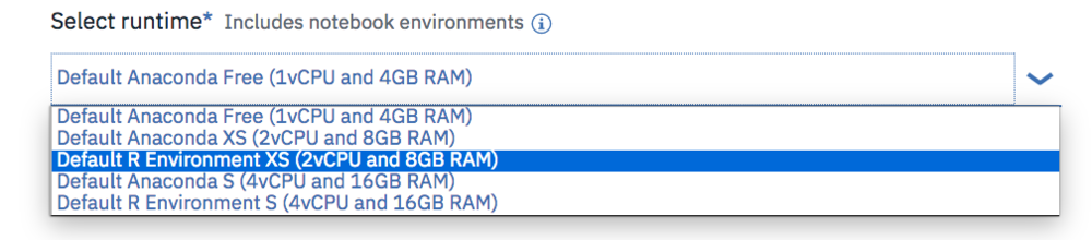
Ensure you select an R environment as the notebook environment.  Click create

For each step below, the instructions are: Create a new cell.  Enter the code below.  Run the code by pressing the top nav button “run cell” which looks like a right arrow. 

Note: If you need to close and reopen your notebook, please make sure to click the edit button in the upper right so that you can interact with the notebook and run the code.

 

Run all the code for steps 1-4 above

1) Install and load the necessary packages

install.packages("ggplot2")
install.packages("data.table")
install.packages("tidyr")

library(ggplot2)
library(data.table)
library(tidyr)

2) Bring in the Austin Imagine Data indicators

#Download the Austin indicator data set
#Original data set from: https://data.austintexas.gov/City-Government/Imagine-Austin-Indicators/apwj-7zty/data
austinData= fread('https://raw.githubusercontent.com/lgellis/MiscTutorial/master/Austin/Imagine_Austin_Indicators.csv', data.table=FALSE, stringsAsFactors = FALSE)

3) Perform some basic data manipulation

We are first going to filter down to only include the “Median Gross Rent” KPI.  After that we need to reformat the table to easily use in a line graph.  Currently the metric value for every year is in it’s own column.  We need to create two new columns to represent the key value pair combination.  

#Attach the column names
attach(austinData)

#Filter to include only Median Gross Rent
aD2 <- austinData[`Indicator Name` == "Median Gross Rent", ]

#Use gather function of tidyr for easier line graph plotting
aD2 <- aD2 %>% 
  gather(year, value, '2007':'2017') 

4) Create a simple chart on one of the key indicators “Median Gross Rent”

#Create a line graph

p <- ggplot(aD2, aes(x=year, y=value, group=1)) + 
  geom_line() +
  labs(x = "Median Gross Rent in Austin",
       y = "Year") +
  theme_bw() + 
  theme_minimal() 

p

5) Export the manipulated data set and chart

This is where things are a little different in the project notesbooks vs hosted RStudio.  On step 5, to export the data from our notebook, we need to use project-lib and insert a special project token.

5a) Go to the project settings.

 

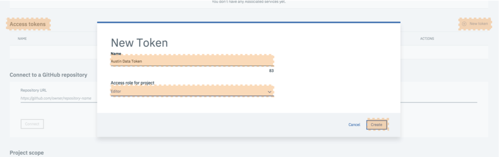
5b) Create the token. 

Select “Access tokens”, “New token”, enter the token info and select “Create”.

 

 

5c) Insert the project token. 

Open back up your project notebook.  Note that you may have to select the little pencil icon again to open it for editing.  Select the more icon in the upper right and then “Insert project token”.  It will then place the project token into the first cell of the notebook.  Run the cell. 

 

5d) Export the data. 

You are now all set up to perform your file exports.  Please start by exporting the data frame to a CSV

#export to csv
write.csv(aD2,"aD2Data.csv")
project$save_data('aD2Data.csv',"aD2Data.csv", overwrite=TRUE)

Export the graph to a PDF

#Export the graph
p + ggsave("aD2LineGraph.pdf")
project$save_data('aD2LineGraph.pdf',"aD2LineGraph.pdf",overwrite=TRUE)

Note that depending on your account type, you may receive an error saying the file was not saved to the project space.  Don’t worry, the files are still stored in your object storage and can be found following steps 5e and 5f below. 

5e) Find the data in object storage

The data is now in your object storage instance.  To navigate there select “Services” in the top navigation and then “Data Services”.  Click on your object storage instance and then click on your bucket.  

 

 

 

5f) Download the files. 

The files should be in your bucket as you named them.  Check the files you want to download and then select “Download objects” 

---

THANK YOU

Thanks for reading along while we learned how to get started with R in Watson Studio.  Please share your thoughts and creations with me on twitter. 

Note that the full code is available on my  github repo.  If you have trouble downloading the file from github, go to the main page of the repo and select “Clone or Download” and then “Download Zip”.