Creating inset maps using spatial objects

< !-- tabsets -->

< !-- code folding -->

First of all, let us attach some packages and data.

# attach packages
library("sp")
library("raster")
library("grid")
library("gridBase")
library("TeachingDemos")
library("rworldmap")
library("RColorBrewer")
library("classInt")

# attach country polygons
data(countriesLow)
cous <- countriesLow
# find the Netherlands
net <- cous[which(cous@data$NAME == "Netherlands"), ]  

# load meuse.riv
data(meuse.riv)
# convert to SpatialPolygons
riv <- SpatialPolygons(list(Polygons(list(Polygon(meuse.riv)), ID = "1")))

# meuse dataset
data(meuse)
coordinates(meuse) <- c("x", "y")
proj4string(meuse) <- CRS("+init=epsg:28992")
# classifying cadmium into 5 classes
q_5 <- classIntervals(meuse@data$cadmium, n = 5, style = "fisher")
pal <- brewer.pal(5, "Reds")
my_cols <- findColours(q_5, pal)
# we also need lat/lon coordinates
meuse_tr <- spTransform(meuse, proj4string(net))

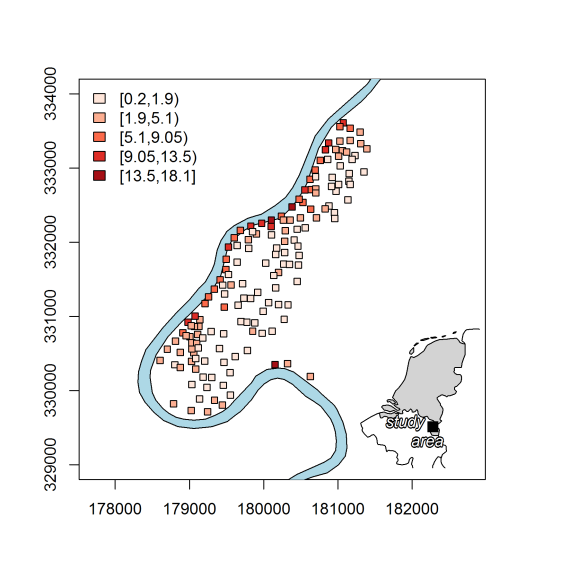
Next, I create the main plot and subsequently add the inset map.

# create the figure
png(file = "meuse.png", w = 1800, h = 1800, res = 300)
plot.new()
vp_1 <- viewport(x = 0, y = 0, width = 0.91, height = 1,
                just = c("left", "bottom"))
vp_2 <- viewport(x = 0.61, y = 0.19, width = 0.22, height = 0.25,
                just = c("left", "bottom"))

# main plot
pushViewport(vp_1)
par(new = TRUE, fig = gridFIG())
plot(raster::crop(riv, bbox(meuse) + c(-500, -1000, 2000, 2000)), axes = TRUE,
     col = "lightblue", xlim = c(178500, 182000), ylim = c(329000, 334000))
plot(meuse, col = "black", bg = my_cols, pch = 22, add = TRUE)
legend("topleft", fill = attr(my_cols, "palette"), 
       legend = names(attr(my_cols, "table")), bty = "n")
upViewport()

# inset map
pushViewport(vp_2)
par(new = TRUE, fig = gridFIG(), mar = rep(0, 4))
# plot the Netherlands and its neighbors
plot(cous[net, ], xlim = c(4.2, 5.8), ylim = c(50, 53.7), 
     col = "white", bg = "transparent")
plot(net, col = "lightgray", add = TRUE)
# add the study area location
points(x = coordinates(meuse_tr)[1, 1], y = coordinates(meuse_tr)[1, 2], 
       cex = 1.5, pch = 15)
shadowtext(x = coordinates(meuse_tr)[1, 1] - 0.35, 
           y = coordinates(meuse_tr)[1, 2] - 0.1,
           labels = "study         \n area",  = 3)
dev.off()