

With the new F1 season upon us, I’ve started tinkering with bits of code from the Wrangling F1 Data With R book and looking at the data in some new ways.
For example, I started wondering whether we might be able to learn something interesting about the race strategies by looking at laptimes on a stint by stint basis.
To begin with, we need some data – I’m going to grab it directly from the ergast API using some functions that are bundled in with the Leanpub book…
#ergast functions described in: https://leanpub.com/wranglingf1datawithr/
#Get laptime data from the ergast API
l2=lapsData.df(2016,2)
#Get pits data from the ergast API
p2=pitsData.df(2016,2)

#merge pit data into the laptime data
l3=merge(l2,p2[,c('driverId','lap','rawduration')],by=c('driverId','lap'),all=T)

#generate an inlap flag (inlap is the lap assigned the pit time)
l3['inlap']=!is.na(l3['rawduration'])

#generate an outlap flag (outlap is the first lap of the race lap's starting from the pits
l3=ddply(l3,.(driverId),transform,outlap=c(T,!is.na(head(rawduration,-1))))

#use the pitstop flag to number stints; note: a drive through penalty increments the stint count
l3=arrange(l3,driverId, -lap)
l3=ddply(l3,.(driverId),transform,stint=1+sum(inlap)-cumsum(inlap))

#number the laps in each stint
l3=arrange(l3,driverId, lap)
l3=ddply(l3,.(driverId,stint),transform,lapInStint=1:length(stint))
l3=arrange(l3,driverId, lap)
The laptimes associated with the in- and out- lap associated with a pit stop add noise to the full lap times completed within each stint, so lets flag those laps so we can then filter them out:
#Discount the inlap and outlap
l4=l3[!l3['outlap'] & !l3['inlap'],]
We can now look at the data… I’m going to facet by driver, and also group the laptimes associated with each stint. Then we can plot just the raw laptimes, and also a simple linear model based on the full lap times within each stint:
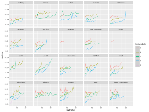
#Generate a base plot
g=ggplot(l4,aes(x=lapInStint, y=rawtime, col=factor(stint)))+facet_wrap(~driverId)

#Chart the raw laptimes within each stint
g+geom_line()

#Plot a simple linear model for each stint
g+ geom_smooth(method = "lm", formula = y ~ x)
So for example, here are the raw laptimes, excluding inlap and outlap, by stint for each driver in the recent 2016 Bahrain Formual One Grand Prix:

And here’s the simple linear model:

These charts highlight several things:
- trivially, the number and length of the stints completed by each driver;
- degradation effects in terms of the gradient of the slope of each stint trace;
- fuel effects- the y-axis offset for each stint is the sum of the fuel effect (as the race progresses the cars get lighter and laptime goes down more or less linearly) and a basic tyre effect (the “base” time we might expect from a tyre). Based on the total number of laps completed in stints prior to a particular stint, we can calculate a fuel effect offset for the laptimes in each stint which should serve to normalise the y-axis laptimes and make more evident the base tyre laptime.
- looking at the charts as a whole, we get a feel for strategy – what sort of tyre/stint strategy do the cars start race with, for example; are the cars going long on tyres without much degradation, or pushing for various length stints on tyres that lose significant time each lap? And so on… (What can you read into/from the charts? Let me know in the comments below;-)
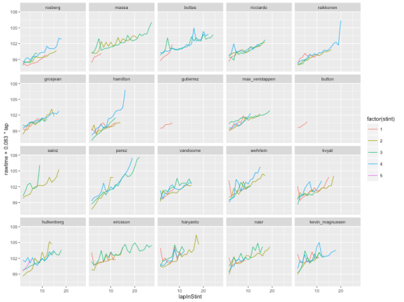
If we assume a 0.083s per lap fuel weight penalty effect, we can replot the chart to account for this:
#Generate a base plot
g=ggplot(l4,aes(x=lapInStint, y=rawtime+0.083*lap, col=factor(stint)))
g+facet_wrap(~driverId) +geom_line()
Here’s what we get:
And here’s what the fuel corrected models look like:

UPDATE: the above fuel calculation goes the wrong way – oops! It should be:
MAXLAPS=max(l4['lap'])
FUEL_PENALTY =0.083
.e = environment()
g=ggplot(l4,aes(x=lapInStint,y=rawtime-(MAXLAPS-lap)*FUEL_PENALTY,col=factor(stint)),environment=.e)
What we really need to do now is annotate the charts with additional tyre selection information for each stint.
We can also do a few more sums. For example, generate a simple average laptime per stint, excluding inlap and outlap times:
#Calculate some stint summary data
l5=ddply(l4,.(driverId,stint), summarise,
                               stintav=sum(rawtime)/length(rawtime),
                               stintsum=sum(rawtime),
                               stinlen=length(rawtime))
which gives results of the form:
          driverId stint   stintav stintsum stinlen
1          rosberg     1  98.04445 1078.489      11
2          rosberg     2  97.55133 1463.270      15
3          rosberg     3  96.15543  673.088       7
4          rosberg     4  96.32494 1637.524      17
5            massa     1  99.13600  495.680       5
6            massa     2 100.48300 2009.660      20
7            massa     3  98.77862 2568.244      26
It would possibly be useful to also compare inlap and outlaps somehow, as well as factoring in the pitstop time. I’m pondering a couple a possibilities for the latter :
- amortise the pitstop time over the laps leading up to a pitstop by adding a pitsop lap penalty to each lap in that stint calculated as the pitstop time of the stint length of the laps in the stint leading up to the pitstop; this essentially penalises the stint that leads up to the pitstop as a consequence of forcing the pitstop;
- amortise the pitstop time over the laps immediately following a pitstop by adding a pitsop lap penalty to each lap in that stint calculated as the pitstop time of the stint length of the laps in the stint following the pitstop; this essentially penalises the stint that immediately follows the pitstop, and discounts some of the benefit from the pitstop.
I haven’t run the numbers yet though, so I’m not sure how these different approaches will feel…

