I hope that Genetics will continue running expository papers about their old classics, like this one by Philip Meneely about Luria & Delbrück (1943). Luria & Delbrück performed an experiment on bacteriophage resistance in Escherichia coli, growing bacterial cultures, exposing them to a phage, and then plating and counting the survivors, who have become resistant to the phage. They considered two hypotheses: either resistance occurs adaptively, in response to the phage, or it occurs by mutation some time during the growth of the culture but before the phages are added. They find the latter to be the case, and this is an example of how mutations happen irrespective of their effects of fitness, in a sense at random. Their analysis is based on a model of bacterial growth and mutation, and the aim of this exercise is to explore this model by simulating some data.

First, we assume that mutation happens with a fixed mutation rate , which is quite close to their estimated value, and that the mutation can’t reverse. We also assume that the bacteria grow by doubling each generation up to 30 generations. We start a culture from a single susceptible bacterium, and let it grow for a number of generations before the phage is added. (We’re going to use discrete generations, while Luria & Delbrück use a continuous function.) Then:

That is, every generation i, the mutants that occur move from the susceptible to the resistant category. The number of mutants that happen among the susceptible is binomially distributed:

.

This is an R function to simulate a culture:

culture <- function(generations, mu) {
  n_susceptible <- numeric(generations)
  n_resistant <- numeric(generations)
  n_mutants <- numeric(generations)
  n_susceptible[1] <- 1
  for (i in 1:(generations - 1)) {
    n_mutants[i] <- rbinom(n = 1, size = n_susceptible[i], prob = mu)
    n_susceptible[i + 1] <- 2 * (n_susceptible[i] - n_mutants[i])
    n_resistant[i + 1] <- 2 * (n_resistant[i] + n_mutants[i])
  }
  data.frame(generation = 1:generations,
             n_susceptible,
             n_resistant,
             n_mutants)
}
cultures <- replicate(1000, culture(30, 2e-8), simplify = FALSE)

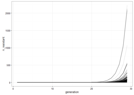
We run a few replicate cultures and plot the number of resistant bacteria. This graph shows the point pretty well: Because of random mutation and exponential growth, the cultures where mutations happen to arise relatively early will give rise to a lot more resistant bacteria than the ones were the first mutations are late. Therefore, there will be a lot of variation between the cultures because of their different histories.

combined <- Reduce(function (x, y) rbind(x, y), cultures)
combined$culture <- rep(1:1000, each = 30)

resistant_plot <- qplot(x = generation, y = n_resistant, group = culture,
      data = combined, geom = "line", alpha = I(1/10), size = I(1)) + theme_bw()

We compare this to what happens under the alternative hypothesis where resistance arises as a consequence of introduction of the phage with some resistance rate (this is not the same as the mutation rate above, even though we’re using the same value). Then the number of resistant cells in a culture will be: .

resistant <- unlist(lapply(cultures, function(x) max(x$n_resistant)))

acquired_resistant <- rbinom(n = 1000, size = 2^29, 2e-8)

resistant_combined <- rbind(transform(data.frame(resistant = acquired_resistant), model = &quot;acquired&quot;),
                            transform(data.frame(resistant = resistant), model = &quot;mutation&quot;))

resistant_histograms <- qplot(x = resistant, data = resistant_combined,bins = 10) +
  facet_wrap(~ model, scale = "free_x")

Here are two histograms side by side to compare the cases. The important thing is the shape. If the acquired resistance hypothesis holds, the number of resistant bacteria in replicate cultures follows a Poisson distribution, because it arises when one counts the number of binomially distributed events that occur in a given number of trials. The interesting thing about the Poisson distribution in this case is that its mean is equal to the variance. However, under the mutation model (as we’ve already illustrated), there is a lot of variation between cultures. These fluctuations make the variance much larger than the mean, which is also what Luria and Delbrück found in their data. Therefore, the results are inconsistent with acquired mutation, and hence the experiment is called the Luria–Delbrück fluctuation test.

mean(resistant)
var(resistant)
mean(acquired_resistant)
var(acquired_resistant)

Literature

Luria, S. E., & Delbrück, M. (1943). Mutations of bacteria from virus sensitivity to virus resistance. Genetics, 28(6), 491.

Meneely, P. M. (2016). Pick Your Poisson: An Educational Primer for Luria and Delbrück’s Classic Paper. Genetics, 202(2), 371-375.

Code on github.