
The Mcomp Package
Want to share your content on R-bloggers? click here if you have a blog, or here if you don't.
Makridakis Competitions (also known as the M Competitions or M-Competitions) are a series of competitions organized by teams led by forecasting researcher Spyros Makridakis and intended to evaluate and compare the accuracy of different forecasting methods. So far three competitions have taken place, named as M1 (1982), M2 (1993) and M3 (2000). The fourth competition is going to take place on year 2018 very soon.
The Mcomp package provides with the set of time series part of the M1 and M3 competitions, specifically 1001 time series from the M1 competition and 3003 from the M3 one.
Packages
suppressPackageStartupMessages(library(Mcomp))
suppressPackageStartupMessages(library(ggplot2))
suppressPackageStartupMessages(library(gridExtra))
suppressPackageStartupMessages(library(Kmisc))
Analysis
The data is provided by the M1 and M3 lists and their summary can be easily printed out.
data(M1)
data(M3)
print(M1)

M-Competition data: 1001 time series

           Type of data
Period      DEMOGR INDUST MACRO1 MACRO2 MICRO1 MICRO2 MICRO3 Total
  MONTHLY       75    183     64     92     10     89    104   617
  QUARTERLY     39     18     45     59      5     21     16   203
  YEARLY        30     35     30     29     16     29     12   181
  Total        144    236    139    180     31    139    132  1001


print(M3)

M-Competition data: 3003 time series

           Type of data
Period      DEMOGRAPHIC FINANCE INDUSTRY MACRO MICRO OTHER Total
  MONTHLY           111     145      334   312   474    52  1428
  OTHER               0      29        0     0     4   141   174
  QUARTERLY          57      76       83   336   204     0   756
  YEARLY            245      58      102    83   146    11   645
  Total             413     308      519   731   828   204  3003
Monthly, quarterly, yearly and some other time aggregation are available (row names) splitted among a pool of data categories (column names).
Each member of the M1 or M3 list is a Mdata object providing with:
-
sn, name of the series
st, series number and period. For example \”Y1\” denotes first yearly series, \”Q20\” denotes 20th quarterly series and so on
n, the number of observations in the time series
h, the number of required forecasts period Interval of the time series.
Possible values are “YEARLY”, “QUARTERLY”, “MONTHLY” & “OTHER”
type, the type of series.
Possible values for M1 are “DEMOGR”, “INDUST”, “MACRO1”, “MACRO2”, “MICRO1”, “MICRO2” & “MICRO3”.
Possible values for M3 are “DEMOGRAPHIC”, “FINANCE”, “INDUSTRY”, “MACRO”, “MICRO”, “OTHER”
description, a short description of the time series
x, a time series of length n (the historical data)
xx, a time series of length h (the future data)
Let us have a look at M1 and M3 first ten elements names.
names(M1)[1:10]

[1] "YAF2"  "YAF3"  "YAF4"  "YAF5"  "YAF6"  "YAF7"  "YAF8"  "YAF9"  "YAF10" "YAF11"


names(M3)[1:10]

[1] "N0001" "N0002" "N0003" "N0004" "N0005" "N0006" "N0007" "N0008" "N0009" "N0010"
Each element is a Mdata S3 class instance. For example:
ts_1 <- M3[["N0001"]]
print(ts_1)

Series: Y1
Type of series: MICRO
Period of series: YEARLY
Series description: SALES ( CODE= ABT)

HISTORICAL data
Time Series:
Start = 1975
End = 1988
Frequency = 1
 [1]  940.66 1084.86 1244.98 1445.02 1683.17 2038.15 2342.52 2602.45 2927.87 3103.96 3360.27
[12] 3807.63 4387.88 4936.99

FUTURE data
Time Series:
Start = 1989
End = 1994
Frequency = 1
[1] 5379.75 6158.68 6876.58 7851.91 8407.84 9156.01
Plots can be achieved by plot() or autoplot() functions, as shown below. The future horizon time series data is plot in red color.
idx <- sample(1:length(M3), 12)
par(mfrow=c(4,3))
invisible(lapply(idx, function(x) { plot(M3[[x]])}))
par(mfrow=c(1,1))
Gives this plot:

plot_list <- invisible(lapply(idx, function(x) { autoplot(M3[[x]])}))
grob_plots <- invisible(lapply(chunk(1, length(plot_list), 12), function(x) {
  marrangeGrob(grobs=lapply(plot_list[x], ggplotGrob), nrow=4, ncol=3)}))
grob_plots
Gives this plot:

We can figure out an helper function that allows the comparison of accuracy and shows resulting plots for the forecasts based on two specified fit methods and parameters. The horizon future is based on the length of future available data. The accuracy is determined by the accuracy() function provided within the forecast package (see refs [4] and [5]).
prepare_arg_list <- function(fit_func, x) {
  func_sig <- names(formals(fit_func))
  arg_list <- list()
  if ("y" %in% func_sig) {
    arg_list <- list(y=x)
  } else if ("data" %in% func_sig) {
    arg_list <- list(data=x)
  } else if ("x" %in% func_sig) {
    arg_list <- list(x=x)
  }
  arg_list
}

analyze_forecast <- function(Mobj, ts_idx, fit_func1, args1 = NULL, fit_func2, args2 = NULL) {
  ts <- Mobj[[ts_idx]]
  x <- ts$x
  xx <- ts$xx
  h <- length(xx)

  arg_list1 <- prepare_arg_list(fit_func1, x)
  model_1 <- do.call(fit_func1, args=c(arg_list1, args1))
  ts_fc_1 <- forecast(model_1, h=h)

  arg_list2 <- prepare_arg_list(fit_func2, x)
  model_2 <- do.call(fit_func2, args=c(arg_list2, args2))
  ts_fc_2 <- forecast(model_2, h=h)

  cat(paste("Accuracy Forecast Method:", substitute(fit_func1), "\n"))
  print(accuracy(ts_fc_1, xx))
  cat("\n")
  cat(paste("Accuracy Forecast Method:", substitute(fit_func2), "\n"))
  print(accuracy(ts_fc_2, xx))

  par(mfrow=c(1,2))

  plot(ts_fc_1)
  lines(xx, col ='red')

  plot(ts_fc_2)
  lines(xx, col='red')

  par(mfrow=c(1,1))

  list(fc1=ts_fc_1, fc2=ts_fc_2)
}
Then we can use it to compare forecast method for a given time series, future horizon and forecast methods. Some examples follows.
Herein below, we compare forecasts generated by ets (exponential smoothing state space model) vs ARIMA auto.arima() function model found. The stepwise = FALSE parameter is passed as input to auto.arima() to allow for a more exhaustive search of candidate models. Both functions are available within forecast package.
analyze_forecast(M3, 1, ets, "ZZZ", auto.arima, list(stepwise=FALSE))

Accuracy Forecast Method: ets
                    ME      RMSE       MAE        MPE     MAPE      MASE
Training set  15.68064  97.95396  81.58716 -0.1594235 3.688927 0.2654018
Test set     445.03563 577.31243 480.61641  5.3426543 6.004038 1.5634378
                  ACF1 Theil's U
Training set 0.1011023        NA
Test set     0.4859372 0.7108304

Accuracy Forecast Method: auto.arima
                    ME      RMSE      MAE      MPE     MAPE      MASE      ACF1
Training set  28.88508  88.49504  68.3793 1.096870 2.439216 0.2224368 0.0146484
Test set     446.25333 578.60264 481.7033 5.358426 6.017378 1.5669735 0.4860139
             Theil's U
Training set        NA
Test set      0.712472
$fc1
     Point Forecast    Lo 80     Hi 80    Lo 95     Hi 95
1989       5486.492 5164.145  5808.839 4993.505  5979.479
1990       6035.932 5300.681  6771.184 4911.463  7160.402
1991       6585.373 5324.965  7845.780 4657.745  8513.000
1992       7134.813 5242.131  9027.495 4240.205 10029.420
1993       7684.253 5053.545 10314.961 3660.932 11707.574
1994       8233.693 4758.261 11709.125 2918.478 13548.908

$fc2
     Point Forecast    Lo 80    Hi 80    Lo 95     Hi 95
1989        5486.10 5363.602 5608.598 5298.756  5673.444
1990        6035.21 5761.297 6309.123 5616.295  6454.125
1991        6584.32 6125.975 7042.665 5883.342  7285.298
1992        7133.43 6462.482 7804.378 6107.303  8159.557
1993        7682.54 6774.072 8591.008 6293.158  9071.922
1994        8231.65 7063.095 9400.205 6444.500 10018.800
Gives this plot:

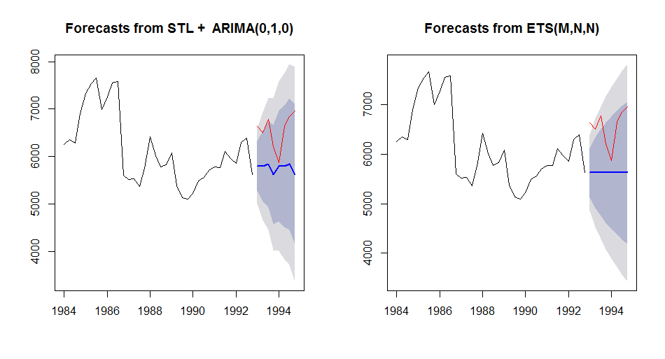
We compare forecast from stlm() with ARIMA model vs stlm() with ets model. The stlm() function is provided within the forecast package. It takes a time series y, applies an STL decomposition, and models the seasonally adjusted data using the model passed as modelfunction or specified using method, in our case arima and ets. The stlm() function returns an object that includes the original STL decomposition and a time series model fitted to the seasonally adjusted data. This object can be passed to the forecast.stlm for forecasting.
analyze_forecast(M3, 700, stlm, list(method=c("arima")), stlm, list(method=c("ets")))

Accuracy Forecast Method: stlm
                    ME     RMSE      MAE        MPE      MAPE      MASE      ACF1 Theil's U
Training set -11.90287 402.5976 252.8155 -0.4288085  4.232485 0.3940372 0.1205458        NA
Test set     792.38609 863.2711 792.3861 11.8446454 11.844645 1.2350097 0.2029283  1.993663

Accuracy Forecast Method: stlm
                    ME     RMSE      MAE        MPE      MAPE      MASE      ACF1 Theil's U
Training set -11.42326 402.6201 253.3089 -0.4211643  4.240385 0.3948063 0.1206962        NA
Test set     792.33085 863.2204 792.3309 11.8438007 11.843801 1.2349236 0.2029283  1.993547
$fc1
        Point Forecast    Lo 80    Hi 80    Lo 95    Hi 95
1993 Q1       5799.191 5275.923 6322.459 4998.921 6599.461
1993 Q2       5796.247 5056.234 6536.260 4664.494 6928.000
1993 Q3       5838.818 4932.490 6745.145 4452.709 7224.926
1993 Q4       5624.900 4578.363 6671.437 4024.360 7225.440
1994 Q1       5799.191 4629.127 6969.255 4009.733 7588.649
1994 Q2       5796.247 4514.506 7077.988 3835.994 7756.500
1994 Q3       5838.818 4454.380 7223.256 3721.502 7956.133
1994 Q4       5624.900 4144.874 7104.926 3361.395 7888.405

$fc2
        Point Forecast    Lo 80    Hi 80    Lo 95    Hi 95
1993 Q1       5799.246 5340.654 6257.838 5097.890 6500.602
1993 Q2       5796.302 5147.163 6445.441 4803.530 6789.075
1993 Q3       5838.873 5043.090 6634.656 4621.828 7055.917
1993 Q4       5624.955 4705.186 6544.724 4218.290 7031.621
1994 Q1       5799.246 4769.926 6828.566 4225.037 7373.456
1994 Q2       5796.302 4667.653 6924.951 4070.183 7522.422
1994 Q3       5838.873 4618.618 7059.128 3972.654 7705.092
1994 Q4       5624.955 4319.189 6930.721 3627.958 7621.952
Gives this plot:

We then compare forecasts based on stlm() with ARIMA vs. ets() ones.
analyze_forecast(M3, 700, stlm, list(method=c("arima")), ets)

Accuracy Forecast Method: stlm
                    ME     RMSE      MAE        MPE      MAPE      MASE      ACF1 Theil's U
Training set -11.90287 402.5976 252.8155 -0.4288085  4.232485 0.3940372 0.1205458        NA
Test set     792.38609 863.2711 792.3861 11.8446454 11.844645 1.2350097 0.2029283  1.993663

Accuracy Forecast Method: ets
                    ME     RMSE     MAE        MPE      MAPE      MASE       ACF1 Theil's U
Training set -38.53996 477.8266 314.552 -0.9081287  5.189619 0.4902595 0.02021015        NA
Test set     932.19799 990.8932 932.198 13.9795463 13.979546 1.4529200 0.25180619  2.285006
$fc1
        Point Forecast    Lo 80    Hi 80    Lo 95    Hi 95
1993 Q1       5799.191 5275.923 6322.459 4998.921 6599.461
1993 Q2       5796.247 5056.234 6536.260 4664.494 6928.000
1993 Q3       5838.818 4932.490 6745.145 4452.709 7224.926
1993 Q4       5624.900 4578.363 6671.437 4024.360 7225.440
1994 Q1       5799.191 4629.127 6969.255 4009.733 7588.649
1994 Q2       5796.247 4514.506 7077.988 3835.994 7756.500
1994 Q3       5838.818 4454.380 7223.256 3721.502 7956.133
1994 Q4       5624.900 4144.874 7104.926 3361.395 7888.405

$fc2
        Point Forecast    Lo 80    Hi 80    Lo 95    Hi 95
1993 Q1       5624.977 5120.941 6129.013 4854.121 6395.833
1993 Q2       5624.977 4911.328 6338.626 4533.545 6716.409
1993 Q3       5624.977 4749.886 6500.068 4286.640 6963.314
1993 Q4       5624.977 4613.281 6636.673 4077.722 7172.232
1994 Q1       5624.977 4492.488 6757.466 3892.984 7356.970
1994 Q2       5624.977 4382.881 6867.073 3725.355 7524.599
1994 Q3       5624.977 4281.718 6968.236 3570.640 7679.314
1994 Q4       5624.977 4187.213 7062.741 3426.107 7823.847
Gives this plot:
We compare forecasts from forecast package tslm() function allowing for trend and seasonality regression and forecasts generated by ets() function.
analyze_forecast(M3, 700, tslm, list(formula = x ~ trend + season), ets)

Accuracy Forecast Method: tslm
                        ME     RMSE       MAE        MPE      MAPE      MASE      ACF1 Theil's U
Training set -5.050281e-14  614.945  535.8089 -0.9563518  8.701461 0.8351095 0.7369323        NA
Test set      1.260770e+03 1313.898 1260.7700 19.0010624 19.001062 1.9650310 0.2691452  3.065128

Accuracy Forecast Method: ets
                    ME     RMSE     MAE        MPE      MAPE      MASE       ACF1 Theil's U
Training set -38.53996 477.8266 314.552 -0.9081287  5.189619 0.4902595 0.02021015        NA
Test set     932.19799 990.8932 932.198 13.9795463 13.979546 1.4529200 0.25180619  2.285006
$fc1
        Point Forecast    Lo 80    Hi 80    Lo 95    Hi 95
1993 Q1       5425.700 4469.084 6382.316 3935.752 6915.648
1993 Q2       5448.222 4491.606 6404.839 3958.275 6938.170
1993 Q3       5441.478 4484.861 6398.094 3951.530 6931.425
1993 Q4       5176.700 4220.084 6133.316 3686.752 6666.648
1994 Q1       5272.460 4297.971 6246.949 3754.676 6790.244
1994 Q2       5294.982 4320.494 6269.471 3777.198 6812.766
1994 Q3       5288.238 4313.749 6262.726 3770.454 6806.022
1994 Q4       5023.460 4048.971 5997.949 3505.676 6541.244

$fc2
        Point Forecast    Lo 80    Hi 80    Lo 95    Hi 95
1993 Q1       5624.977 5120.941 6129.013 4854.121 6395.833
1993 Q2       5624.977 4911.328 6338.626 4533.545 6716.409
1993 Q3       5624.977 4749.886 6500.068 4286.640 6963.314
1993 Q4       5624.977 4613.281 6636.673 4077.722 7172.232
1994 Q1       5624.977 4492.488 6757.466 3892.984 7356.970
1994 Q2       5624.977 4382.881 6867.073 3725.355 7524.599
1994 Q3       5624.977 4281.718 6968.236 3570.640 7679.314
1994 Q4       5624.977 4187.213 7062.741 3426.107 7823.847
Gives this plot:

Further, the Mcomp package makes available forecasts produced by M3 competitors and benchmarks as provided by the M3Forecast list. Hereinbelow the name of M3 competitors and benchmarks.
names(M3Forecast)

 [1] "NAIVE2"       "SINGLE"       "HOLT"         "DAMPEN"       "WINTER"       "COMB S-H-D"
 [7] "B-J auto"     "AutoBox1"     "AutoBox2"     "AutoBox3"     "ROBUST-Trend" "ARARMA"
[13] "Auto-ANN"     "Flors-Pearc1" "Flors-Pearc2" "PP-Autocast"  "ForecastPro"  "SMARTFCS"
[19] "THETAsm"      "THETA"        "RBF"          "ForcX"        "AAM1"         "AAM2"
A helper function allows evaluating the accuracy of those forecasts.
m3_competition_accuracy <- function(ts_idx, competitorName, plot=FALSE) {
  v <- na.omit(as.numeric(M3Forecast[[competitorName]][ts_idx,]))
  xx <- M3[[ts_idx]]$xx
  sn <- M3[[ts_idx]]$sn
  v_ts <- ts(v, frequency = frequency(xx), start = start(xx))

  if (plot) {
    plot(M3[[ts_idx]], main = sn)
    legend("topleft", legend = c("Actual", competitorName), fill = c("red", "blue"))
    lines(v_ts, col = 'blue')
  }

  accuracy(v_ts, xx)
}
Herein below some examples.
m3_competition_accuracy(150, "HOLT", TRUE)

               ME     RMSE      MAE        MPE     MAPE      ACF1 Theil's U
Test set 571.4183 2130.361 1913.418 -0.1041563 32.05945 0.5902855  1.721647
Gives this plot:

m3_competition_accuracy(150, "ROBUST-Trend", TRUE)

               ME    RMSE     MAE      MPE     MAPE      ACF1 Theil's U
Test set 923.1167 2108.68 1762.95 7.199077 27.50348 0.5838244  1.512274
Gives this plot:

Conclusions
Mcomp package represents a valuable resource for time series analysis. There is also available the Tcomp package providing with 1311 time series of class Mcomp from the tourism forecasting competition conducted in 2010.
If you have any questions, please feel free to comment below.
References
- [1] Mcomp package vignette
[2] Tcomp package vignette
[3] Makridakis Competitions
[4] Forecast package
[5] Evaluating Forecast Accuracy, Prof. Rob J. Hyndman
Related Post
- Building a Hacker News scraper with 8 lines of R code using rvest library
- Building a Telecom Dictionary scraping web using rvest in R
- Scraping Javascript-rendered web content using R
- Analysing Cryptocurrency Market in R
- Time Series Analysis in R Part 3: Getting Data from Quandl
R-bloggers.com offers daily e-mail updates about R news and tutorials about learning R and many other topics. Click here if you're looking to post or find an R/data-science job.
Want to share your content on R-bloggers? click here if you have a blog, or here if you don't.