
The Generalized Lambda Distribution and GLDEX Package for Fitting Financial Return Data – Part 2
Want to share your content on R-bloggers? click here if you have a blog, or here if you don't.
Part 2 of a series
by Daniel Hanson, with contributions by Steve Su (author of the GLDEX package)
Recap of Part 1
In our previous article, we introduced the four-parameter Generalized Lambda Distribution (GLD) and looked at fitting a 20-year set of returns from the Wilshire 5000 Index, comparing the results of two methods, namely the Method of Moments, and the Method of Maximum Likelihood.
Errata: One very important omission in Part 1, however, was not putting
require(GLDEX)
prior to the examples shown. Many thanks to a reader who pointed this out in the comments section last time.
Let’s also recall the code we used for obtaining returns from the Wilshire 5000 index, and the first four moments of the data (details are in Part 1):
require(quantmod) # quantmod package must be installed
getSymbols(“VTSMX”, from = “1994-09-01”)
VTSMX.Close <- VTSMX[,4] # Closing prices
VTSMX.vector <- as.vector(VTSMX.Close)
# Calculate log returns
Wilsh5000 <- diff(log(VTSMX.vector), lag = 1)
Wilsh5000 <- 100 * Wilsh5000[-1] # Remove the NA in the first position,
# and put in percent format
# Moments of Wilshire 5000 market returns:
fun.moments.r(Wilsh5000,normalise=”Y”) # normalise=”Y” — subtracts the 3
# from the normal dist value.
# Results:
# mean variance skewness kurtosis
# 0.02824676 1.50214916 -0.30413445 7.82107430
Finally, in Part 1, we looked at two methods for fitting a GLD to this data, namely the Method of Moments (MM), and the Method of Maximum Likelihood (ML). We found that MM gave us a near perfect match in mean, variance, skewness, and kurtosis, but goodness of fit measures showed that we could not conclude that the market data was drawn from the fitted distribution. On the other hand, ML gave us a much better fit, but it came at the price of skewness being way off compared to that of the data, and kurtosis not being determined by the fitting algorithm (NA).
Method of L-Moments (LM)
Steve Su, in his contributions to this article series, suggested the option of a “third way”, namely the Method of L-Moments. Also, as mentioned in the paper L-moments and TL-moments of the generalized lambda distribution, (William H. Asquith, 2006),
“The method of L-moments is an alternative technique, which is suitable and popular for heavy-tailed distributions. The method of L-moments is particularly useful for distributions, such as the generalized lambda distribution (GLD), that are only expressible in inverse or quantile function form.”
Additional details on the method and algorithm for computing it can be found in this paper, noted above.
As we will see in the example that follows, the result is essentially a compromise between our first two results, but the goodness of fit is still far preferable to that of the Method of Moments.
We follow the same approach as above, but using the GLDEX function fun.RMFMKL.lm(.) to calculate the fitted distribution:
# Fit the LM distribution:
require(GLDEX) # Remembered it this time!
wshLambdaLM = fun.RMFMKL.lm(Wilsh5000)
# Compute the associated moments
fun.theo.mv.gld(wshLambdaLM[1], wshLambdaLM[2], wshLambdaLM[3], wshLambdaLM[4],
param = “fmkl”, normalise=”Y”)
# The results are:
# mean variance skewness kurtosis
# 0.02824678 1.56947022 -1.32265715 291.58852044
As was the case with the maximum likelihood fit, the mean and variance are reasonably close, but the skewness and kurtosis do not match the empirical data. However, the skew is not as far off as in the ML case, and we are at least able to calculate a kurtosis value.
Looking at our goodness of fit tests based on the KS statistic:
fun.diag.ks.g(result = wshLambdaLM, data = Wilsh5000, no.test = 1000,
param = “fmkl”)
# Result: 740/1000
ks.gof(Wilsh5000,”pgl”, wshLambdaLM, param=”fmkl”)
# D = 0.0201, p-value = 0.03383
In the first case, our result of 740/1000 suggests a much better fit than the Method of Moments (53/1000) in Part 1, while falling slightly from the ratio we obtained with the Method of Maximum Likelihood. In the second test, a p-value of 0.03383 is not overwhelmingly convincing, but technically it does allow us to accept the hypothesis that our data is drawn from the same distribution at an α = 0.025 or 0.01 confidence level.
Perhaps more interesting is just looking at the plot
bins <- nclass.FD(Wilsh5000) # We get 158 (Freedman-Diaconis Rule)
fun.plot.fit(fit.obj = wshLambdaLM, data = Wilsh5000, nclass = bins, param = “fmkl”,
xlab = “Returns”, main = “Method of L-Moments”)
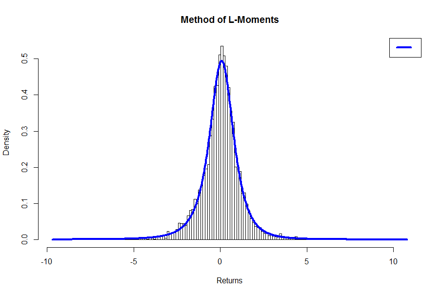
Again, compared to the result for the Method of Moments in Part 1, the plot suggests that we have a better fit.
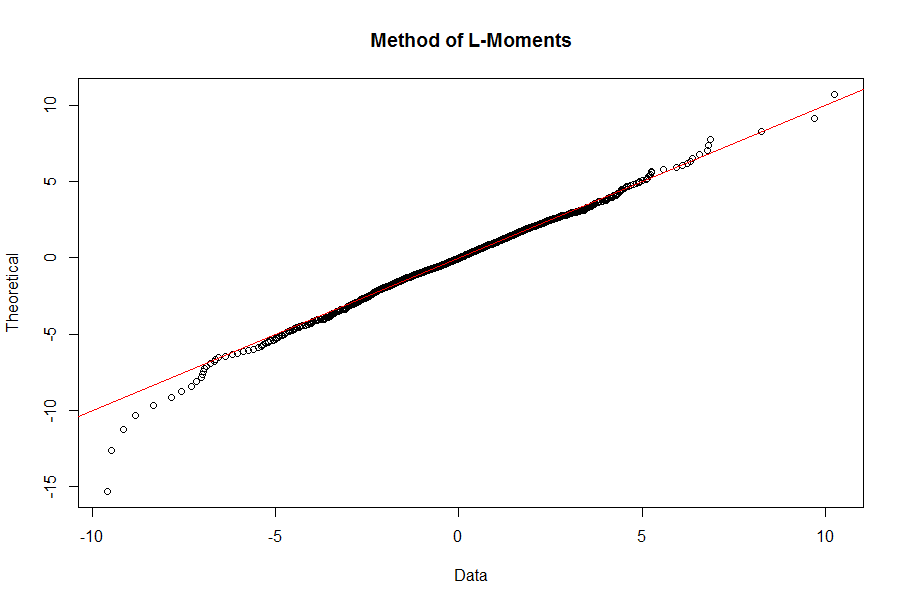
The QQ plot, however, is not much different than what we got in the Maximum Likelihood case; in particular, losses in the left tail are not underestimated by the fitted distribution as they are in the MM case:
qqplot.gld(fit=wshLambdaLM,data=Wilsh5000,param=”fkml”, type = “str.qqplot”,
main = “Method of L-Moments”)
Which Option is “Best”?
Steve Su points out that there is no one “best” solution, as there are trade-offs and competing constraints involved in the algorithms, and it is one reason why, in addition to the methods described above, so many different functions are available in the GLDEX package. On one point, however, there is general agreement in the literature, and that is the Method of Moments — even with the appeal of matching the moments of the empirical data — is an inferior method to others that result in a better fit. This is also discussed in the paper by Asquith, namely, that the method of moments “generally works well for light-tailed distributions. For heavy-tailed distributions, however, use of the method of moments can be questioned.”
Comparison with the Normal Distribution
For a strawman comparison, we can fit the Wilshire 5000 returns to a normal distribution in R, and run the KS test as follows:
f <- fitdistr(Wilsh5000, densfun = "normal")
ks.test(Wilsh5000, “pnorm”, f$estimate[1], f$estimate[2], alternative = “two.sided”)
The results are as follows:
# One-sample Kolmogorov-Smirnov test
# data: Wilsh5000
# D = D = 0.0841, p-value < 2.2e-16
# alternative hypothesis: two-sided
With a p-value that small, we can firmly reject the returns data as being drawn from a fitted normal distribution.
We can also get a look at the plot of the implied normal distribution overlaid upon the fit we obtained with the method of L-moments, as follows:
x <- seq(min(Wilsh5000), max(Wilsh5000), bins)
# Chop the domain into bins = 158nintervals to get sample points
# from the approximated normal distribution (Freedman-Diaconis)
fun.plot.fit(fit.obj = wshLambdaLM, data = Wilsh5000, nclass = bins,
param = “fmkl”, xlab = “Returns”)
curve(dnorm(x, mean=f$estimate[1], sd=f$estimate[2]), add=TRUE,
col = “red”, lwd = 2) # Normal curve in red
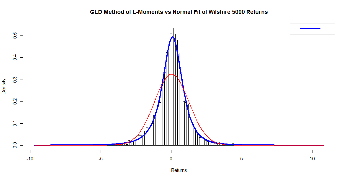
Although it may be a little difficult to see, note that between -3 and -4 on the horizontal axis, the tail of the normal fit (in red) falls below that of the GLD (in blue), and it is along this left tail where extreme events can occur in the markets. The normal distribution implies a lower probability of these “black swan” events than the more representative GLD.
This is further confirmed by looking at the QQ plot vs a normal distribution fit. Note how the theoretical fit (horizontal axis in this case, using the Base R function qqnorm(.); ie, the axes are switched compared to those in our previous QQ plots) vastly underestimates losses in the left tail.
qqnorm(Wilsh5000, main = “Normal Q-Q Plot”)
qqline(Wilsh5000)
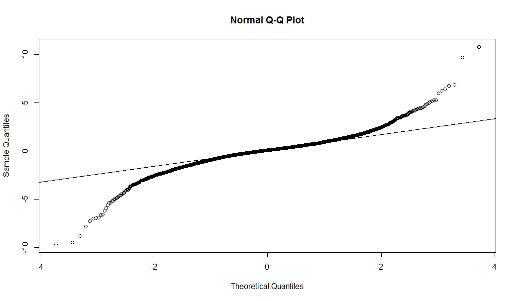
In summary, from these plots, we can see that the GLD fit, particularly using ML or LM, is a superior alternative to what we get with the normal distribution fit when estimating potential index losses.
Conclusion
We have seen, using R and the GLDEX package, how a four parameter distribution such as the Generalized Lambda Distribution can be used to fit a more realistic distribution to market data as compared to the normal distribution, particularly considering the fat tails typically present in returns data that cannot be captured by a normal distribution. While the Method of Moments as a fitting algorithm is highly appealing due to its preserving the moments of the empirical distribution, we sacrifice goodness of fit that can be obtained using other methods such as Maximum Likelihood, and L-Moments.
The GLD has been demonstrated in financial texts and research literature as a suitable distributional fit for determining market risk measures such as Value at Risk (VaR), Expected Shortfall (ES), and other metrics. We will look at examples in an upcoming article.
Again, very special thanks are due to Dr Steve Su for his contributions and guidance in presenting this topic.
R-bloggers.com offers daily e-mail updates about R news and tutorials about learning R and many other topics. Click here if you're looking to post or find an R/data-science job.
Want to share your content on R-bloggers? click here if you have a blog, or here if you don't.