
Practical Machine Learning with R and Python – Part 2
Want to share your content on R-bloggers? click here if you have a blog, or here if you don't.
In this 2nd part of the series “Practical Machine Learning with R and Python – Part 2”, I continue where I left off in my first post Practical Machine Learning with R and Python – Part 2. In this post I cover the some classification algorithmns and cross validation. Specifically I touch
-Logistic Regression
-K Nearest Neighbors (KNN) classification
-Leave out one Cross Validation (LOOCV)
-K Fold Cross Validation
in both R and Python.
As in my initial post the algorithms are based on the following courses.
- Statistical Learning, Prof Trevor Hastie & Prof Robert Tibesherani, Online Stanford
- Applied Machine Learning in Python Prof Kevyn-Collin Thomson, University Of Michigan, Coursera
You can download this R Markdown file along with the data from Github. I hope these posts can be used as a quick reference in R and Python and Machine Learning.I have tried to include the coolest part of either course in this post.
The following classification problem is based on Logistic Regression. The data is an included data set in Scikit-Learn, which I have saved as csv and use it also for R. The fit of a classification Machine Learning Model depends on how correctly classifies the data. There are several measures of testing a model’s classification performance. They are
–Accuracy = TP + TN / (TP + TN + FP + FN) – Fraction of all classes correctly classified
–Precision = TP / (TP + FP) – Fraction of correctly classified positives among those classified as positive
– Recall = TP / (TP + FN) Also known as sensitivity, or True Positive Rate (True positive) – Fraction of correctly classified as positive among all positives in the data
– F1 = 2 * Precision * Recall / (Precision + Recall)
1a. Logistic Regression – R code
The caret and e1071 package is required for using the confusionMatrix call
source("RFunctions.R")
library(dplyr)
library(caret)
library(e1071)
# Read the data (from sklearn)
cancer <- read.csv("cancer.csv")
# Rename the target variable
names(cancer) <- c(seq(1,30),"output")
# Split as training and test sets
train_idx <- trainTestSplit(cancer,trainPercent=75,seed=5)
train <- cancer[train_idx, ]
test <- cancer[-train_idx, ]

# Fit a generalized linear logistic model,
fit=glm(output~.,family=binomial,data=train,control = list(maxit = 50))
# Predict the output from the model
a=predict(fit,newdata=train,type="response")
# Set response >0.5 as 1 and <=0.5 as 0
b=ifelse(a>0.5,1,0)
# Compute the confusion matrix for training data
confusionMatrix(b,train$output)
## Confusion Matrix and Statistics
##
##           Reference
## Prediction   0   1
##          0 154   0
##          1   0 272
##
##                Accuracy : 1
##                  95% CI : (0.9914, 1)
##     No Information Rate : 0.6385
##     P-Value [Acc > NIR] : < 2.2e-16
##
##                   Kappa : 1
##  Mcnemar's Test P-Value : NA
##
##             Sensitivity : 1.0000
##             Specificity : 1.0000
##          Pos Pred Value : 1.0000
##          Neg Pred Value : 1.0000
##              Prevalence : 0.3615
##          Detection Rate : 0.3615
##    Detection Prevalence : 0.3615
##       Balanced Accuracy : 1.0000
##
##        'Positive' Class : 0
##
m=predict(fit,newdata=test,type="response")
n=ifelse(m>0.5,1,0)
# Compute the confusion matrix for test output
confusionMatrix(n,test$output)
## Confusion Matrix and Statistics
##
##           Reference
## Prediction  0  1
##          0 52  4
##          1  5 81
##
##                Accuracy : 0.9366
##                  95% CI : (0.8831, 0.9706)
##     No Information Rate : 0.5986
##     P-Value [Acc > NIR] : <2e-16
##
##                   Kappa : 0.8677
##  Mcnemar's Test P-Value : 1
##
##             Sensitivity : 0.9123
##             Specificity : 0.9529
##          Pos Pred Value : 0.9286
##          Neg Pred Value : 0.9419
##              Prevalence : 0.4014
##          Detection Rate : 0.3662
##    Detection Prevalence : 0.3944
##       Balanced Accuracy : 0.9326
##
##        'Positive' Class : 0
##
1b. Logistic Regression – Python code
import numpy as np
import pandas as pd
import os
import matplotlib.pyplot as plt
from sklearn.model_selection import train_test_split
from sklearn.linear_model import LogisticRegression
os.chdir("C:\\Users\\Ganesh\\RandPython")
from sklearn.datasets import make_classification, make_blobs

from sklearn.metrics import confusion_matrix
from matplotlib.colors import ListedColormap
from sklearn.datasets import load_breast_cancer
# Load the cancer data
(X_cancer, y_cancer) = load_breast_cancer(return_X_y = True)
X_train, X_test, y_train, y_test = train_test_split(X_cancer, y_cancer,
                                                   random_state = 0)
# Call the Logisitic Regression function
clf = LogisticRegression().fit(X_train, y_train)
fig, subaxes = plt.subplots(1, 1, figsize=(7, 5))
# Fit a model
clf = LogisticRegression().fit(X_train, y_train)

# Compute and print the Accuray scores
print('Accuracy of Logistic regression classifier on training set: {:.2f}'
     .format(clf.score(X_train, y_train)))
print('Accuracy of Logistic regression classifier on test set: {:.2f}'
     .format(clf.score(X_test, y_test)))
y_predicted=clf.predict(X_test)
# Compute and print confusion matrix
confusion = confusion_matrix(y_test, y_predicted)
from sklearn.metrics import accuracy_score, precision_score, recall_score, f1_score
print('Accuracy: {:.2f}'.format(accuracy_score(y_test, y_predicted)))
print('Precision: {:.2f}'.format(precision_score(y_test, y_predicted)))
print('Recall: {:.2f}'.format(recall_score(y_test, y_predicted)))
print('F1: {:.2f}'.format(f1_score(y_test, y_predicted)))
## Accuracy of Logistic regression classifier on training set: 0.96
## Accuracy of Logistic regression classifier on test set: 0.96
## Accuracy: 0.96
## Precision: 0.99
## Recall: 0.94
## F1: 0.97
2. Dummy variables
The following R and Python code show how dummy variables are handled in R and Python. Dummy variables are categorival variables which have to be converted into appropriate values before using them in Machine Learning Model For e.g. if we had currency as ‘dollar’, ‘rupee’ and ‘yen’ then the dummy variable will convert this as
dollar 0 0 0
rupee 0 0 1
yen 0 1 0
2a. Logistic Regression with dummy variables- R code
# Load the dummies library
library(dummies)
df <- read.csv("adult1.csv",stringsAsFactors = FALSE,na.strings = c(""," "," ?"))

# Remove rows which have NA
df1 <- df[complete.cases(df),]
dim(df1)
## [1] 30161    16
# Select specific columns
adult <- df1 %>% dplyr::select(age,occupation,education,educationNum,capitalGain,
                               capital.loss,hours.per.week,native.country,salary)
# Set the dummy data with appropriate values
adult1 <- dummy.data.frame(adult, sep = ".")

#Split as training and test
train_idx <- trainTestSplit(adult1,trainPercent=75,seed=1111)
train <- adult1[train_idx, ]
test <- adult1[-train_idx, ]

# Fit a binomial logistic regression
fit=glm(salary~.,family=binomial,data=train)
# Predict response
a=predict(fit,newdata=train,type="response")
# If response >0.5 then it is a 1 and 0 otherwise
b=ifelse(a>0.5,1,0)
confusionMatrix(b,train$salary)
## Confusion Matrix and Statistics
##
##           Reference
## Prediction     0     1
##          0 16065  3145
##          1   968  2442
##
##                Accuracy : 0.8182
##                  95% CI : (0.8131, 0.8232)
##     No Information Rate : 0.753
##     P-Value [Acc > NIR] : < 2.2e-16
##
##                   Kappa : 0.4375
##  Mcnemar's Test P-Value : < 2.2e-16
##
##             Sensitivity : 0.9432
##             Specificity : 0.4371
##          Pos Pred Value : 0.8363
##          Neg Pred Value : 0.7161
##              Prevalence : 0.7530
##          Detection Rate : 0.7102
##    Detection Prevalence : 0.8492
##       Balanced Accuracy : 0.6901
##
##        'Positive' Class : 0
##
# Compute and display confusion matrix
m=predict(fit,newdata=test,type="response")
## Warning in predict.lm(object, newdata, se.fit, scale = 1, type =
## ifelse(type == : prediction from a rank-deficient fit may be misleading
n=ifelse(m>0.5,1,0)
confusionMatrix(n,test$salary)
## Confusion Matrix and Statistics
##
##           Reference
## Prediction    0    1
##          0 5263 1099
##          1  357  822
##
##                Accuracy : 0.8069
##                  95% CI : (0.7978, 0.8158)
##     No Information Rate : 0.7453
##     P-Value [Acc > NIR] : < 2.2e-16
##
##                   Kappa : 0.4174
##  Mcnemar's Test P-Value : < 2.2e-16
##
##             Sensitivity : 0.9365
##             Specificity : 0.4279
##          Pos Pred Value : 0.8273
##          Neg Pred Value : 0.6972
##              Prevalence : 0.7453
##          Detection Rate : 0.6979
##    Detection Prevalence : 0.8437
##       Balanced Accuracy : 0.6822
##
##        'Positive' Class : 0
##
2b. Logistic Regression with dummy variables- Python code
Pandas has a get_dummies function for handling dummies
import numpy as np
import pandas as pd
import os
import matplotlib.pyplot as plt
from sklearn.model_selection import train_test_split
from sklearn.linear_model import LogisticRegression
from sklearn.metrics import confusion_matrix
from sklearn.metrics import accuracy_score, precision_score, recall_score, f1_score
# Read data
df =pd.read_csv("adult1.csv",encoding="ISO-8859-1",na_values=[""," "," ?"])
# Drop rows with NA
df1=df.dropna()
print(df1.shape)
# Select specific columns
adult = df1[['age','occupation','education','educationNum','capitalGain','capital-loss',
             'hours-per-week','native-country','salary']]

X=adult[['age','occupation','education','educationNum','capitalGain','capital-loss',
             'hours-per-week','native-country']]
# Set approporiate values for dummy variables
X_adult=pd.get_dummies(X,columns=['occupation','education','native-country'])
y=adult['salary']

X_adult_train, X_adult_test, y_train, y_test = train_test_split(X_adult, y,
                                                   random_state = 0)
clf = LogisticRegression().fit(X_adult_train, y_train)

# Compute and display Accuracy and Confusion matrix
print('Accuracy of Logistic regression classifier on training set: {:.2f}'
     .format(clf.score(X_adult_train, y_train)))
print('Accuracy of Logistic regression classifier on test set: {:.2f}'
     .format(clf.score(X_adult_test, y_test)))
y_predicted=clf.predict(X_adult_test)
confusion = confusion_matrix(y_test, y_predicted)
print('Accuracy: {:.2f}'.format(accuracy_score(y_test, y_predicted)))
print('Precision: {:.2f}'.format(precision_score(y_test, y_predicted)))
print('Recall: {:.2f}'.format(recall_score(y_test, y_predicted)))
print('F1: {:.2f}'.format(f1_score(y_test, y_predicted)))
## (30161, 16)
## Accuracy of Logistic regression classifier on training set: 0.82
## Accuracy of Logistic regression classifier on test set: 0.81
## Accuracy: 0.81
## Precision: 0.68
## Recall: 0.41
## F1: 0.51
3a – K Nearest Neighbors Classification – R code
The Adult data set is taken from UCI Machine Learning Repository
source("RFunctions.R")
df <- read.csv("adult1.csv",stringsAsFactors = FALSE,na.strings = c(""," "," ?"))
# Remove rows which have NA
df1 <- df[complete.cases(df),]
dim(df1)
## [1] 30161    16
# Select specific columns
adult <- df1 %>% dplyr::select(age,occupation,education,educationNum,capitalGain,
                               capital.loss,hours.per.week,native.country,salary)
# Set dummy variables
adult1 <- dummy.data.frame(adult, sep = ".")

#Split train and test as required by KNN classsification model
train_idx <- trainTestSplit(adult1,trainPercent=75,seed=1111)
train <- adult1[train_idx, ]
test <- adult1[-train_idx, ]
train.X <- train[,1:76]
train.y <- train[,77]
test.X <- test[,1:76]
test.y <- test[,77]

# Fit a model for 1,3,5,10 and 15 neighbors
cMat <- NULL
neighbors <-c(1,3,5,10,15)
for(i in seq_along(neighbors)){
    fit =knn(train.X,test.X,train.y,k=i)
    table(fit,test.y)
    a<-confusionMatrix(fit,test.y)
    cMat[i] <- a$overall[1]
    print(a$overall[1])
}
##  Accuracy
## 0.7835831
##  Accuracy
## 0.8162047
##  Accuracy
## 0.8089113
##  Accuracy
## 0.8209787
##  Accuracy
## 0.8184591
#Plot the Accuracy for each of the KNN models
df <- data.frame(neighbors,Accuracy=cMat)
ggplot(df,aes(x=neighbors,y=Accuracy)) + geom_point() +geom_line(color="blue") +
    xlab("Number of neighbors") + ylab("Accuracy") +
    ggtitle("KNN regression - Accuracy vs Number of Neighors (Unnormalized)")

3b – K Nearest Neighbors Classification – Python code
import numpy as np
import pandas as pd
import os
import matplotlib.pyplot as plt
from sklearn.model_selection import train_test_split
from sklearn.metrics import confusion_matrix
from sklearn.metrics import accuracy_score, precision_score, recall_score, f1_score
from sklearn.neighbors import KNeighborsClassifier
from sklearn.preprocessing import MinMaxScaler
# Read data
df =pd.read_csv("adult1.csv",encoding="ISO-8859-1",na_values=[""," "," ?"])
df1=df.dropna()
print(df1.shape)
# Select specific columns
adult = df1[['age','occupation','education','educationNum','capitalGain','capital-loss',
'hours-per-week','native-country','salary']]
X=adult[['age','occupation','education','educationNum','capitalGain','capital-loss',
'hours-per-week','native-country']]
#Set values for dummy variables
X_adult=pd.get_dummies(X,columns=['occupation','education','native-country'])
y=adult['salary']
X_adult_train, X_adult_test, y_train, y_test = train_test_split(X_adult, y,
random_state = 0)
# KNN classification in Python requires the data to be scaled.
# Scale the data
scaler = MinMaxScaler()
X_train_scaled = scaler.fit_transform(X_adult_train)
# Apply scaling to test set also
X_test_scaled = scaler.transform(X_adult_test)
# Compute the KNN model for 1,3,5,10 & 15 neighbors
accuracy=[]
neighbors=[1,3,5,10,15]
for i in neighbors:
knn = KNeighborsClassifier(n_neighbors = i)
knn.fit(X_train_scaled, y_train)
accuracy.append(knn.score(X_test_scaled, y_test))
print('Accuracy test score: {:.3f}'
.format(knn.score(X_test_scaled, y_test)))
# Plot the models with the Accuracy attained for each of these models
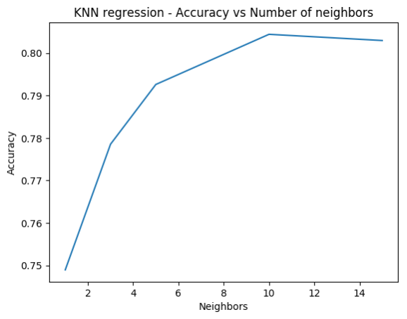
fig1=plt.plot(neighbors,accuracy)
fig1=plt.title("KNN regression - Accuracy vs Number of neighbors")
fig1=plt.xlabel("Neighbors")
fig1=plt.ylabel("Accuracy")
fig1.figure.savefig('foo1.png', bbox_inches='tight')
## (30161, 16)
## Accuracy test score: 0.749
## Accuracy test score: 0.779
## Accuracy test score: 0.793
## Accuracy test score: 0.804
## Accuracy test score: 0.803
Output image:
4 MPG vs Horsepower
The following scatter plot shows the non-linear relation between mpg and horsepower. This will be used as the data input for computing K Fold Cross Validation Error
4a MPG vs Horsepower scatter plot – R Code
df=read.csv("auto_mpg.csv",stringsAsFactors = FALSE) # Data from UCI
df1 <- as.data.frame(sapply(df,as.numeric))
df2 <- df1 %>% dplyr::select(cylinder,displacement, horsepower,weight, acceleration, year,mpg)
df3 <- df2[complete.cases(df2),]
ggplot(df3,aes(x=horsepower,y=mpg)) + geom_point() + xlab("Horsepower") +
    ylab("Miles Per gallon") + ggtitle("Miles per Gallon vs Hosrsepower")

4b MPG vs Horsepower scatter plot – Python Code
import numpy as np
import pandas as pd
import os
import matplotlib.pyplot as plt
autoDF =pd.read_csv("auto_mpg.csv",encoding="ISO-8859-1")
autoDF.shape
autoDF.columns
autoDF1=autoDF[['mpg','cylinder','displacement','horsepower','weight','acceleration','year']]
autoDF2 = autoDF1.apply(pd.to_numeric, errors='coerce')
autoDF3=autoDF2.dropna()
autoDF3.shape
#X=autoDF3[['cylinder','displacement','horsepower','weight']]
X=autoDF3[['horsepower']]
y=autoDF3['mpg']

fig11=plt.scatter(X,y)
fig11=plt.title("KNN regression - Accuracy vs Number of neighbors")
fig11=plt.xlabel("Neighbors")
fig11=plt.ylabel("Accuracy")
fig11.figure.savefig('foo11.png', bbox_inches='tight')

5 K Fold Cross Validation
K Fold Cross Validation is a technique in which the data set is divided into K Folds or K partitions. The Machine Learning model is trained on K-1 folds and tested on the Kth fold i.e.
we will have K-1 folds for training data and 1 for testing the ML model. Since we can partition this as 
Validation estimates the average validation error that we can expect on a new unseen test data.
The formula for K Fold Cross validation is as follows
and
and
^{2}}{n_{K}}")

 MSE_{K}")
where 

Leave Out one Cross Validation (LOOCV) is a special case of K Fold Cross Validation where N-1 data points are used to train the model and 1 data point is used to test the model. There are N such paritions of N-1 & 1 that are possible. The mean error is measured The Cross Valifation Error for LOOCV is

where 
^{2}}{1-h_{i}}")
see [Statistical Learning]
The above formula is also included in this blog post
It took me a day and a half to implement the K Fold Cross Validation formula. I think it is correct. In any case do let me know if you think it is off
5a. Leave out one cross validation (LOOCV) – R Code
R uses the package ‘boot’ for performing Cross Validation error computation
library(boot)
library(reshape2)
# Read data
df=read.csv("auto_mpg.csv",stringsAsFactors = FALSE) # Data from UCI
df1 <- as.data.frame(sapply(df,as.numeric))
# Select complete cases
df2 <- df1 %>% dplyr::select(cylinder,displacement, horsepower,weight, acceleration, year,mpg)
df3 <- df2[complete.cases(df2),]
set.seed(17)
cv.error=rep(0,10)
# For polynomials 1,2,3... 10 fit a LOOCV model
for (i in 1:10){
    glm.fit=glm(mpg~poly(horsepower,i),data=df3)
    cv.error[i]=cv.glm(df3,glm.fit)$delta[1]

}
cv.error
##  [1] 24.23151 19.24821 19.33498 19.42443 19.03321 18.97864 18.83305
##  [8] 18.96115 19.06863 19.49093
# Create and display a plot
folds <- seq(1,10)
df <- data.frame(folds,cvError=cv.error)
ggplot(df,aes(x=folds,y=cvError)) + geom_point() +geom_line(color="blue") +
    xlab("Degree of Polynomial") + ylab("Cross Validation Error") +
    ggtitle("Leave one out Cross Validation - Cross Validation Error vs Degree of Polynomial")

5b. Leave out one cross validation (LOOCV) – Python Code
In Python there is no available function to compute Cross Validation error and we have to compute the above formula. I have done this after several hours. I think it is now in reasonable shape. Do let me know if you think otherwise. For LOOCV I use the K Fold Cross Validation with K=N
import numpy as np
import pandas as pd
import os
import matplotlib.pyplot as plt
from sklearn.linear_model import LinearRegression
from sklearn.cross_validation import train_test_split, KFold
from sklearn.preprocessing import PolynomialFeatures
from sklearn.metrics import mean_squared_error
# Read data
autoDF =pd.read_csv("auto_mpg.csv",encoding="ISO-8859-1")
autoDF.shape
autoDF.columns
autoDF1=autoDF[['mpg','cylinder','displacement','horsepower','weight','acceleration','year']]
autoDF2 = autoDF1.apply(pd.to_numeric, errors='coerce')
# Remove rows with NAs
autoDF3=autoDF2.dropna()
autoDF3.shape
X=autoDF3[['horsepower']]
y=autoDF3['mpg']

# For polynomial degree 1,2,3... 10
def computeCVError(X,y,folds):
    deg=[]
    mse=[]
    degree1=[1,2,3,4,5,6,7,8,9,10]

    nK=len(X)/float(folds)
    xval_err=0
    # For degree 'j'
    for j in degree1:
        # Split as 'folds'
        kf = KFold(len(X),n_folds=folds)
        for train_index, test_index in kf:
            # Create the appropriate train and test partitions from the fold index
            X_train, X_test = X.iloc[train_index], X.iloc[test_index]
            y_train, y_test = y.iloc[train_index], y.iloc[test_index]

            # For the polynomial degree 'j'
            poly = PolynomialFeatures(degree=j)
            # Transform the X_train and X_test
            X_train_poly = poly.fit_transform(X_train)
            X_test_poly = poly.fit_transform(X_test)
            # Fit a model on the transformed data
            linreg = LinearRegression().fit(X_train_poly, y_train)
            # Compute yhat or ypred
            y_pred = linreg.predict(X_test_poly)
            # Compute MSE * n_K/N
            test_mse = mean_squared_error(y_test, y_pred)*float(len(X_train))/float(len(X))
            # Add the test_mse for this partition of the data
            mse.append(test_mse)
        # Compute the mean of all folds for degree 'j'
        deg.append(np.mean(mse))

    return(deg)


df=pd.DataFrame()
print(len(X))
# Call the function once. For LOOCV K=N. hence len(X) is passed as number of folds
cvError=computeCVError(X,y,len(X))

# Create and plot LOOCV
df=pd.DataFrame(cvError)
fig3=df.plot()
fig3=plt.title("Leave one out Cross Validation - Cross Validation Error vs Degree of Polynomial")
fig3=plt.xlabel("Degree of Polynomial")
fig3=plt.ylabel("Cross validation Error")
fig3.figure.savefig('foo3.png', bbox_inches='tight')

6a K Fold Cross Validation – R code
Here K Fold Cross Validation is done for 4, 5 and 10 folds using the R package boot and the glm package
library(boot)
library(reshape2)
set.seed(17)
#Read data
df=read.csv("auto_mpg.csv",stringsAsFactors = FALSE) # Data from UCI
df1 <- as.data.frame(sapply(df,as.numeric))
df2 <- df1 %>% dplyr::select(cylinder,displacement, horsepower,weight, acceleration, year,mpg)
df3 <- df2[complete.cases(df2),]
a=matrix(rep(0,30),nrow=3,ncol=10)
set.seed(17)
# Set the folds as 4,5 and 10
folds<-c(4,5,10)
for(i in seq_along(folds)){
    cv.error.10=rep(0,10)
    for (j in 1:10){
        # Fit a generalized linear model
        glm.fit=glm(mpg~poly(horsepower,j),data=df3)
        # Compute K Fold Validation error
        a[i,j]=cv.glm(df3,glm.fit,K=folds[i])$delta[1]

    }

}

# Create and display the K Fold Cross Validation Error
b <- t(a)
df <- data.frame(b)
df1 <- cbind(seq(1,10),df)
names(df1) <- c("PolynomialDegree","4-fold","5-fold","10-fold")

df2 <- melt(df1,id="PolynomialDegree")
ggplot(df2) + geom_line(aes(x=PolynomialDegree, y=value, colour=variable),size=2) +
    xlab("Degree of Polynomial") + ylab("Cross Validation Error") +
    ggtitle("K Fold Cross Validation - Cross Validation Error vs Degree of Polynomial")

6b. K Fold Cross Validation – Python code
The implementation of K-Fold Cross Validation Error has to be implemented and I have done this below. There is a small discrepancy in the shapes of the curves with the R plot above. Not sure why!
import numpy as np
import pandas as pd
import os
import matplotlib.pyplot as plt
from sklearn.linear_model import LinearRegression
from sklearn.cross_validation import train_test_split, KFold
from sklearn.preprocessing import PolynomialFeatures
from sklearn.metrics import mean_squared_error
# Read data
autoDF =pd.read_csv("auto_mpg.csv",encoding="ISO-8859-1")
autoDF.shape
autoDF.columns
autoDF1=autoDF[['mpg','cylinder','displacement','horsepower','weight','acceleration','year']]
autoDF2 = autoDF1.apply(pd.to_numeric, errors='coerce')
# Drop NA rows
autoDF3=autoDF2.dropna()
autoDF3.shape
#X=autoDF3[['cylinder','displacement','horsepower','weight']]
X=autoDF3[['horsepower']]
y=autoDF3['mpg']

# Create Cross Validation function
def computeCVError(X,y,folds):
    deg=[]
    mse=[]
    # For degree 1,2,3,..10
    degree1=[1,2,3,4,5,6,7,8,9,10]

    nK=len(X)/float(folds)
    xval_err=0
    for j in degree1:
        # Split the data into 'folds'
        kf = KFold(len(X),n_folds=folds)
        for train_index, test_index in kf:
            # Partition the data acccording the fold indices generated
            X_train, X_test = X.iloc[train_index], X.iloc[test_index]
            y_train, y_test = y.iloc[train_index], y.iloc[test_index]

            # Scale the X_train and X_test as per the polynomial degree 'j'
            poly = PolynomialFeatures(degree=j)
            X_train_poly = poly.fit_transform(X_train)
            X_test_poly = poly.fit_transform(X_test)
            # Fit a polynomial regression
            linreg = LinearRegression().fit(X_train_poly, y_train)
            # Compute yhat or ypred
            y_pred = linreg.predict(X_test_poly)
            # Compute MSE *(nK/N)
            test_mse = mean_squared_error(y_test, y_pred)*float(len(X_train))/float(len(X))
            # Append to list for different folds
            mse.append(test_mse)
        # Compute the mean for poylnomial 'j'
        deg.append(np.mean(mse))

    return(deg)

# Create and display a plot of K -Folds
df=pd.DataFrame()
for folds in [4,5,10]:
    cvError=computeCVError(X,y,folds)
    #print(cvError)
    df1=pd.DataFrame(cvError)
    df=pd.concat([df,df1],axis=1)
    #print(cvError)

df.columns=['4-fold','5-fold','10-fold']
df=df.reindex([1,2,3,4,5,6,7,8,9,10])
df
fig2=df.plot()
fig2=plt.title("K Fold Cross Validation - Cross Validation Error vs Degree of Polynomial")
fig2=plt.xlabel("Degree of Polynomial")
fig2=plt.ylabel("Cross validation Error")
fig2.figure.savefig('foo2.png', bbox_inches='tight')
output

This concludes this 2nd part of this series. I will look into model tuning and model selection in R and Python in the coming parts. Comments, suggestions and corrections are welcome!
To be continued….
Watch this space!
Also see
- Design Principles of Scalable, Distributed Systems
- Re-introducing cricketr! : An R package to analyze performances of cricketers
- Spicing up a IBM Bluemix cloud app with MongoDB and NodeExpress
- Using Linear Programming (LP) for optimizing bowling change or batting lineup in T20 cricket
- Simulating an Edge Shape in Android
To see all posts see Index of posts

R-bloggers.com offers daily e-mail updates about R news and tutorials about learning R and many other topics. Click here if you're looking to post or find an R/data-science job.
Want to share your content on R-bloggers? click here if you have a blog, or here if you don't.