
Package lconnect: patch connectivity metrics and patch prioritization
Want to share your content on R-bloggers? click here if you have a blog, or here if you don't.
Today we are presenting a new package, lconnect. This package is intended to be a very simple approach to derive landscape connectivity metrics. Many of these metrics come from the interpretation of landscape as graphs.
Additionally, it also provides a function to prioritize landscape patches based on their contribution to the overall landscape connectivity. For now this function works only with the Integral Index of connectivity, by Pascual-Hortal & Saura (2006).
For now we only have a development version in GitHub, but a more definitive version should be uploaded to CRAN in the coming days.
Here’s a brief tutorial!
First install the package:
#load package from GitHub
#install.packages("devtools")
#remove.packages("lconnect", lib="~/R/win-library/3.5")
library(devtools)
install_github("FMestre1/lconnect")
library(lconnect)
Then, upload the landscape shapefile …
#Load data
vec_path <- system.file("extdata/vec_projected.shp", package = "lconnect")
…and create a ‘lconnect’ class object:
#upload landscape
land <- upload_land(vec_path, habitat = 1, max_dist = 500)
class(land)
## [1] "lconnect"
And now, let’s plot it:
plot(land, main="Landscape clusters")

If we wish we can derive patch importance (the contribution of each individual patch to the overall connectivity):
land1 <- patch_imp(land, metric="IIC")
##  [1]  0.0000000  0.0000000  0.0000000  0.0000000  0.0000000  0.1039501
##  [7]  0.1039501  0.0000000  0.1039501  0.0000000  0.0000000  0.1039501
## [13]  0.3118503 21.9334719  0.0000000 15.5925156  2.5987526  0.1039501
## [19]  0.1039501  0.2079002  0.0000000  0.0000000  0.0000000  0.0000000
## [25]  0.9355509  0.0000000 14.2411642  2.9106029  0.2079002 12.9937630
## [31]  0.3118503  0.7276507  0.0000000  7.5883576  0.5197505 70.2702703
class(land1)
Which produces an object of the class ‘pimp’:
## [1] "pimp"
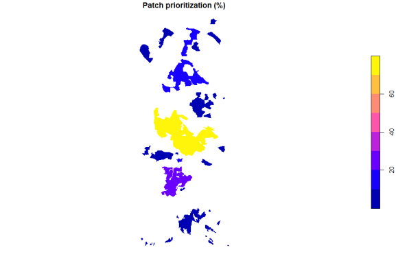
And, finally, we can also plot the relative contribution of each patch to the landscape connectivity:
plot(land1, main="Patch prioritization (%)")
And that’s it!
R-bloggers.com offers daily e-mail updates about R news and tutorials about learning R and many other topics. Click here if you're looking to post or find an R/data-science job.
Want to share your content on R-bloggers? click here if you have a blog, or here if you don't.