
Marginal Effects for (mixed effects) regression models #rstats
Want to share your content on R-bloggers? click here if you have a blog, or here if you don't.
ggeffects (CRAN, website) is a package that computes marginal effects at the mean (MEMs) or representative values (MERs) for many different models, including mixed effects or Bayesian models. One of the advantages of the package is its easy-to-use interface: No matter if you fit a simple or complex model, with interactions or splines, the function call is always the same. This also holds true for the returned output, which is always a data frame with the same, consistent column names.
The past package-update introduced some new features I wanted to describe here: a revised print()-method as well as a new opportunity to plot marginal effects at different levels of random effects in mixed models…
The new print()-method
The former print()-method simply showed the first predicted values, including confidence intervals. For numeric predictor variables with many values, you could, for instance, only see the first 10 of more than 100 predicted values. While it makes sense to shorten the (console-)output, there was no information about the predictions for the last or other „representative“ values of the term in question. Now, the print()-method automatically prints a selection of representative values, so you get a quick and clean impression of the range of predicted values for continuous variables:
library(ggeffects)
data(efc)
efc$c172code <- as.factor(efc$c172code)
fit <- lm(barthtot ~ c12hour * c172code + neg_c_7, data = efc)

ggpredict(fit, "c12hour")
#>
#> # Predicted values of Total score BARTHEL INDEX
#> # x = average number of hours of care per week
#>
#>    x predicted std.error conf.low conf.high
#>    0    72.804     2.516   67.872    77.736
#>   20    68.060     2.097   63.951    72.170
#>   45    62.131     1.824   58.555    65.706
#>   65    57.387     1.886   53.691    61.083
#>   85    52.643     2.179   48.373    56.913
#>  105    47.900     2.626   42.752    53.047
#>  125    43.156     3.164   36.955    49.357
#>  170    32.482     4.531   23.602    41.363
#>
#> Adjusted for:
#> * c172code =     1
#> *  neg_c_7 = 11.83
If you print predicted values of a term, grouped by the levels of another term (which makes sense in the above example due to the present interaction), the print()-method automatically adjusts the range of printed values to keep the console-output short. In the following example, only 6 instead of 8 values per „block“ are shown:
ggpredict(fit, c("c12hour", "c172code"))
#>
#> # Predicted values of Total score BARTHEL INDEX
#> # x = average number of hours of care per week
#>
#> # c172code = 1
#>    x predicted std.error conf.low conf.high
#>    0    72.804     2.516   67.872    77.736
#>   30    65.689     1.946   61.874    69.503
#>   55    59.759     1.823   56.186    63.331
#>   85    52.643     2.179   48.373    56.913
#>  115    45.528     2.887   39.870    51.186
#>  170    32.482     4.531   23.602    41.363
#>
#> # c172code = 2
#>    x predicted std.error conf.low conf.high
#>    0    76.853     1.419   74.073    79.633
#>   30    68.921     1.115   66.737    71.106
#>   55    62.311     1.122   60.112    64.510
#>   85    54.379     1.438   51.560    57.198
#>  115    46.447     1.934   42.656    50.238
#>  170    31.905     3.007   26.011    37.800
#>
#> # c172code = 3
#>    x predicted std.error conf.low conf.high
#>    0    73.862     2.502   68.958    78.766
#>   30    66.925     1.976   63.053    70.798
#>   55    61.145     2.155   56.920    65.369
#>   85    54.208     2.963   48.400    60.016
#>  115    47.271     4.057   39.320    55.222
#>  170    34.554     6.303   22.200    46.907
#>
#> Adjusted for:
#> * neg_c_7 = 11.83
Marginal effects at specific levels of random effects
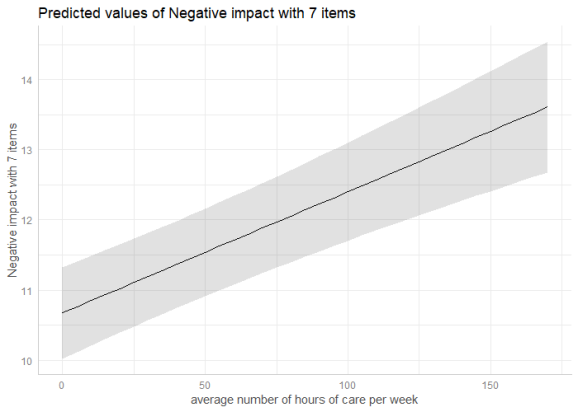
Marginal effects can also be calculated for each group level in mixed models. Simply add the name of the related random effects term to the terms-argument, and set type = "re". In the following example, we fit a linear mixed model and first simply plot the marginal effetcs, not conditioned on random effects.
library(sjlabelled)
library(lme4)
data(efc)
efc$e15relat <- as_label(efc$e15relat)
m <- lmer(neg_c_7 ~ c12hour + c160age + c161sex + (1 | e15relat), data = efc)
me <- ggpredict(m, terms = "c12hour")
plot(me)
To compute marginal effects for each grouping level, add the related random term to the terms-argument. In this case, confidence intervals are not calculated, but marginal effects are conditioned on each group level of the random effects.
me <- ggpredict(m, terms = c("c12hour", "e15relat"), type = "re")
plot(me)

Marginal effects, conditioned on random effects, can also be calculated for specific levels only. Add the related values into brackets after the variable name in the terms-argument.
me <- ggpredict(m, terms = c("c12hour", "e15relat [child,cousin]"), type = "re")
plot(me)

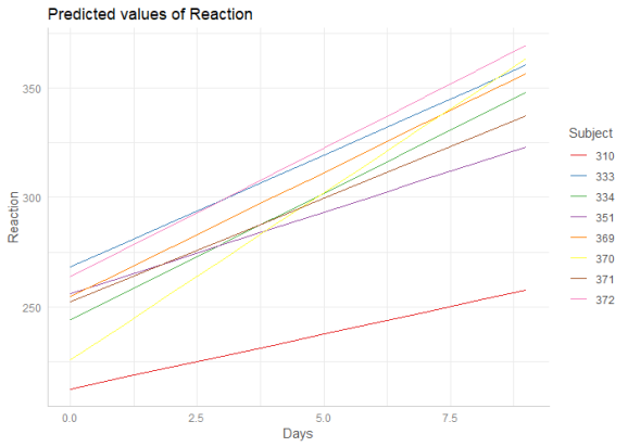
If the group factor has too many levels, you can also take a random sample of all possible levels and plot the marginal effects for this subsample of group levels. To do this, use term = "groupfactor [sample=n]".
data("sleepstudy")
m <- lmer(Reaction ~ Days + (1 + Days | Subject), data = sleepstudy)
me <- ggpredict(m, terms = c("Days", "Subject [sample=8]"), type = "re")
plot(me)
R-bloggers.com offers daily e-mail updates about R news and tutorials about learning R and many other topics. Click here if you're looking to post or find an R/data-science job.
Want to share your content on R-bloggers? click here if you have a blog, or here if you don't.