This post explains a two-stage stochastic linear programming (SLP) in a simplified manner and implements this model using R. This exercise is for the clear understanding of SLP model and will be a solid basis for the advanced topics such as multi-stage SLP, scenario tree generation, and so on.


For 2-stage SLP, we use the simple ALM cash flow matching problem which was dealt with the following previous post.

Stochastic Linear Programming

Stochastic programming assumes that some given parameters (i.e. interest rates, liabilities requirements) in deterministic model are random variables with known probability distributions. Of course, there are also predetermined or known parameters in SLP.

For example, in the floating rate note, the first coupon rate is predetermined prior to a pricing date but the remaining coupon rates are going to be realized at the future reset dates so that our decisions for subsequent buying, selling, and holding will be dependent on these realizations.

As a whole, SLP is classified either as two-stage SLP or multi-stage SLP. The former has two decision timings and the latter has multiple decision times. More realistic model is also multi-stage SLP but as you know, dealing with many stages all at once is much more difficult than only two-stage.

In practice and academics, multi-stage and two-stage or three-stage SLP are widely used. In some case, multi-stage SLP can be converted into a two-stage SLP. Before delving into the advanced multi-stage SLP model, it is natural that our focus centers on two-stage SLP at first.

From the following figure, we can find that 1) sky blue circle in the first stage is known and shows one realization but 2) grey circles in the second stage are not known and show possible realizations with probabilities (a set of scenario).


Figure : Illustration of two-stage stochastic programming

The first decision must be made here-and-now and cannot depend on future realizations. The second decision is the wait-and-see decision which can be made after some of the random parameters are observed. In the sense that the second decision has a characteristics of correction after seeing data, this type of SLP is called the recourse model. We interpret the recourse as a correction.

We think that this kind of reasoning is in line with the Kalman filtering process which consists of alternating repetitions of a prediction and a correction. Prediction is done without observing data and correction after seeing data.

A Generic Form of Two-stage SLP Problem with Recourse

A generic form of a two-stage SLP program with recourse has the following form.

\[\begin{align} &\max_{x} a^T x + E[\max_{y(\omega)} c(\omega)^Ty(\omega)] \\ s.t. &\\ & Ax = b \\ & B(\omega)x + C(\omega)y(\omega) = d(\omega) \\ &x \ge 0, \quad y(\omega) \ge 0 \end{align}\]
In the above formulation, the objective function consists of a decision of \(x\) and expectation of decision of \(y(\omega)\). When \(x\) is found by optimization, future scenarios are used as the form of expectation because we do not know which scenario is revealed but know the probability of each scenario, which can be summarized by the expectation.

Constraint for \(x\) is set with deterministic parameters independently of the future scenario. But constraints for \(y(\omega)\) are set with stochastic parameters and it is affected by a decision of \(x\) because resource is not infinite.

Deterministic Equivalent of Two-stage SLP Problem with Recourse

When probabilities of scenarios are discrete, \[\begin{align} E[\max_{y(\omega)} c(w)^Ty(\omega)] = \sum_{k=1}^{S} {p_k \max_{y(\omega_k)} c(\omega_k)^Ty(\omega_k) } \end{align}\]
Using a notation \(_k\) instead of the \((\omega_k)\), the two-stage SLP problem has the following discretized form.
\[\begin{align} &\max_{x} a^T x + \sum_{k=1}^{S} {p_k \max_{y_k} c_k^Ty_k } \\ s.t. &\\ & Ax = b \\ & B_k x + C_k y_k = d_k \quad k = 1,…,S \\ &x \ge 0 \\ &y_k \ge 0 \quad k = 1,…,S \end{align}\]
For an implementation, we can expand summation into each components as follows.
Constraint for \(x\) is set with deterministic parameters independently of the future scenario. But constraints for \(y(\omega)\) are set with stochastic parameters and it is affected by a decision of \(x\) because resource is not infinite.

Introduction of Interest Rate Scenario

Stohcastic scenario is vital to SLP modeling. Scenario generation can be applied to Interest rates, stock returns, liability cash flows, and so on. For interest rate scenarios, Black-Derman-Toy (BDT) model is widely used.

For a simplified interet rate scenarios. we add two possible interest rate scenarios to the simple ALM cash flow matching problem which was dealt with the previous post.

In the next figure for scenario, interest rates for two-stage consist of the case of up and down and we assume that the interest rates of CP funding are all above the interest rates of the line of credit. This view is intended for investigating the substitution effect between the line of credit and CP funding.


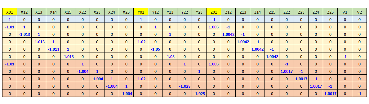
Let \(X\) denote a vector of 25 decision variables, three 1st-stage decision variables (\(x_{01}, y_{01}, z_{01}\)) and the rest of 2nd-stage decision variables, and then the following representation can be obtained.
\[\begin{align} &\max_{X} 0.5\nu_1 + 0.5\nu_2 \\ s.t. &\\ &AX = b \\ \\ &X \ge 0, \quad x_{01}, x_{1i}, x_{2i} \le 100 \\ \\ X = &x_{01}, x_{12},x_{13},x_{14},x_{15},x_{22},x_{23},x_{24},x_{25}, \\ &y_{01},y_{12},y_{13},y_{22},y_{23},\\ &z_{01},z_{12},z_{13},z_{14},z_{15},z_{22},z_{23},z_{24},z_{25}, \\ &v_{1},v_{2} \end{align}\]
Here, the constraint matrix (\(A\)) has the following form. Now we can solve this problem by using R.

R code

In this post, we use ROI and ROI.plugin.lpsolve R packages to solve the above linear optimization problem locally instead of ROI.plugin.neos. The following R code implements the above simplified two-stage stochastic linear programming for the same asset-liability cash flow matching problem with the help of ROI and ROI.plugin.lpsolve.




Comparing this result with the previous one, we can find that ALM manager try to use more funding of the line of credit than the previous deterministic case because future funding cost for the line of credit is relatively cheaper than that of CP issuance. Since we use the equality constraints, the first decision is not changed but the latter decisions are affected by the future interest rate scenarios.

Concluding Remarks

In this post, we implements the two-stage SLP for the simple ALM cash flow matching model. However, we need to be cautious about this implementation. Our problem is so simple that we can use naïve LP programming. But more realistic SLP models have highly dimensional scenario structures so that it can not be solved this naïve method. For solving the realistic two-stage or multi-stage SLP, many advanced numerical techniques are presented and commercial solvers such as GAMS, CPLEX are used.

Keep in mind that our simplified example is for the clear understanding of two-stage stochastic linear programming as a building block for the next advanced model.\(\blacksquare\)