I want to consider an approach of forecasting I really like and frequently use. It allows to include the promo campaigns (or another activities and other variables as well) effect into the prediction of total amount. I will use a fictitious example and data in this post, but it works really good with my real data.  So, you can adapt this algorithm for your requirements and test it. Also, it seems simple for non-math people because of complete automation.

Suppose we sell some service and our business depends on the number of subscribers we attract. Definitely, we measure the number of customers and want to predict their quantity. If we know the customer’s life time value (CLV) it allows us to predict the total revenue based on quantity of customers and CLV. So, this case looks like justified.

The first way we can use for solving this problem is multiple regression. We can find a great number of relevant indicators which influence the number of subscribers. It can be service price, seasonality, promotional activities, even S&P or Dow Jones index, etc. After we found all parameters affecting number of customers we can calculate formula and predict number of customers.

This approach has disadvantages:

• we should collect all these indicators in one place and have historical data of all of them,
• they should be measured at the same time intervals,
• most importantly, we should predict all of these indicators as well. If our customers buy several different packages of our service and for different periods, even our average price doesn’t look like it can be easily predicted (not mentioning S&P index). If we use predicted indicators, their prediction errors will affect the final prediction as well.

On the other hand, stock market analysts use time-series forecasting. They are resigned by the fact that stock prices are influenced by a great number of indicators. Thus, they are looking for dependence inside the price curve. This approach is not fully suitable for us too. In case we regularly attracted extra customers via promos (we can see some peaks on curve) the time-series algorithms can identify peaks as seasonality and draw future curve with the same peaks, but what we can do if we are not planning promos in these periods or we are going to make extra promos or change their intensity.

And final statement before we start working on our prediction algorithm. I’m sure it is important for marketers to see how their promos or activities affect the number of customers / revenue (or subscribers in our case).

So, our task is to create the model which doesn’t depend on a great number of predictors from one side (looks like time-series forecasting) and on the other side includes promos effect on total number of subscribers from the other side (looks like regression).

My answer is extended ARIMA model. ARIMA is Auto Regression Integrated Moving Average. “Extended” means we can include some other information in time-series forecasting based on ARIMA model. In our case, other information is the result of promos we had and we are going to get in the future. In case we repeat promo campaigns every year at the same period and get approximately the same number of new customers ARIMA model (not extended) would be enough. It should recognize peaks as a seasonality. This example we won’t review.

Let’s start. Suppose our data is:

We have (from the left to the right):

• # of period,
• year,
• month,
• number of subscribers,
• monthly growth (difference between number of subscribers in the next month and number of subscribers in the previous month),
• extended (sum of promos effect),
• several types of promo campaigns which affected the number of customers (promo1, promo2, etc.). Also, you can see that some subscribers from particular promo are gone (negative number). When we run some special low pricing promos we realize that part of these customers won’t extend their subscriptions. So, this is the example which includes negative effect of promo campaigns as well.

We need only two variables to make the prediction (‘growth’ and ‘extended’). There are other variables just for your information. Also we have two last months without number of subscribers (we are going to predict these values), but we should have promos effect which we are planning to get in future. Further, the heat-map of growth and extended variables look alike. Thus, we can make conclusion that they are connected.

In the example we will predict values from the 37th to the 42nd to see accuracy of prediction on factual data.

The code in R can be the next:

#load libraries
library(forecast)
library(TSA)
#load data set
df <- read.csv(file='data.csv')
#define periods (convenient for future, you can just change values for period you want to predict or include to factual)
s.date <- c(2010,1)    #start date - factual
e.date <- c(2011,12)   #end date - factual
f.s.date <- c(2013,1)  #start date - prediction
f.e.date <- c(2013,12) #end date - prediction


#transform values to time-series and define past and future periods
growth <- ts(df$Growth, start=s.date, end=e.date, frequency=12)
ext <- ts(df$Extended, start=s.date, end=f.e.date, frequency=12)
past <- window(ext, s.date, e.date)
future <- window(ext, f.s.date, f.e.date)

#ARIMA model
fit <- auto.arima(growth, xreg=past, stepwise=FALSE, approximation=FALSE) #determine model
forecast <- forecast(fit, xreg=future) #make prediction
plot(forecast) #plot chart
summary(forecast) #print predicted values

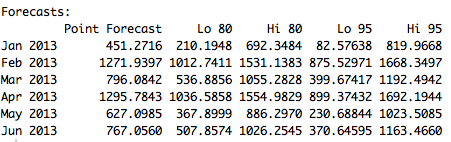
We should get chart and values:

As you remember we have factual data for Jan.2013-Apr.2013 which we can compare: 384 vs 451, 1224 vs 1271, 709 vs 796 and 699 vs 753. Although values are not very close, we can see that February promo affected and we saw a peak. After we add Jan.2013-Mar.2013 to factual periods, our prediction for April will be 718 which is closer to 699 than 753. That means once we have factual data we should recalculate and precise the prediction.

Thus, we have predicted number of subscribers including promo campaigns effect. If we are not satisfied with this number we can add some activity and measure new prediction. Suppose we add new activity for attracting 523 new customers in April 2013 (this means Extended will be 500 instead of -23). In this case our prediction will be:

We got the new peak 1295 in April instead of 753 (in previous prediction). Thus, we have tool for targeting number of subscribers, the only thing we need is to attract these subscribers which we are going to use for prediction ;).

Note, for making prediction for more periods just add values of extended variable in the initial data and change prediction period in the R code.

In case when described approach works poorly I can recommend you this great book written by ‘forecast’ package creator prof. Rob J Hyndman to deepen into forecasting.

Have an accurate predictions!