
How to make a precision recall curve in R
Want to share your content on R-bloggers? click here if you have a blog, or here if you don't.
Precision recall (PR) curves are useful for machine learning model evaluation when there is an extreme imbalance in the data and the analyst is interested particuarly in one class. A good example is credit card fraud, where the instances of fraud are extremely few compared with non fraud. Here are some facts about PR curves.
- PR curves are sensitive to which class is defined as positive, unlike the ROC curve which is a more balanced method. So we will get a completely different result depending on which class is set as positive.
- PR curves are sensitive to class distribution, so if the ratio of positives to negatives changes across different analyses, then the PR curve cannot be used to compare performance between them. This is because the chance line varies between datasets with different class distributions.
- PR curves, because they use precision, instead of specificity (like ROC) can pick up false positives in the predicted positive fraction. This is very helpful when negatives >> positives. In these cases, the ROC is pretty insensitive and can be misleading, whereas PR curves reign supreme.
- The area under the PR curve does not have a probabilistic interpretation like ROC.
The PR gain curve was made to deal with some of the above problems with PR curves, although it still is intended for extreme class imbalance situations. The main difference is the PR gain curve has a universal baseline as precision is corrected according to chance expectation. We will see this in an example.
Note, we are using non repeated cross validation with Caret to save time, but it requires repeating generally to reduce the variance and bias. Also, for imbalanced data in Caret we need to change to the ‘prSummary’ function that uses area under the PR curve to select the best model.
MLeval (https://cran.r-project.org/web/packages/MLeval/index.html) makes curves and calculates metrics, and will automatically extract the best model parameters and data from the Caret results.
## load libraries required for analysis
library(MLeval)
library(caret)

## simulate data
im <- twoClassSim(2000, intercept = -25, linearVars = 20)
table(im$Class)

## run caret
fitControl <- trainControl(method = "cv",summaryFunction=prSummary,
classProbs=T,savePredictions = T,verboseIter = F)
im_fit <- train(Class ~ ., data = im,method = "ranger",metric = "AUC",
trControl = fitControl)
im_fit2 <- train(Class ~ ., data = im,method = "xgbTree",metric = "AUC",
trControl = fitControl)

## run MLeval
x <- evalm(list(im_fit,im_fit2))

## curves and metrics are in the 'x' list object
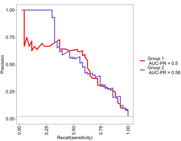
We can see in the below analyses, both models are above chance and xgbTree does slightly better than random forest. Pretty cool.
This is the PR curve, see the grey line is baseline chance expectation.
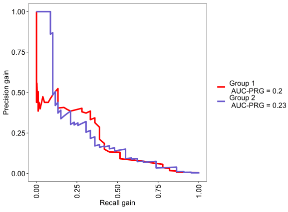
This is the PR gain curve, where baseline is zero.
R-bloggers.com offers daily e-mail updates about R news and tutorials about learning R and many other topics. Click here if you're looking to post or find an R/data-science job.
Want to share your content on R-bloggers? click here if you have a blog, or here if you don't.