Introduction

This article is also available in PDF form.

A while back someone posted on Reddit about the grading policies of their academic department. Specifically, the department chair made a statement claiming that grades should be Normally distributed with a C average. I responded, claiming that no statistician would ever take the idea that grades follow a Normal distribution seriously. Some asked for context, and I wrote a long response explaining my position. I repeat that argument here, and also give some R code demonstrations showing what curving grades does.

Grades Are Not Naturally Normal

A cheap shot would be to say that Normal random variables have no minimum or maximum so since there is a minimum or maximum grade, grades cannot be Normally distributed. This is a cheap shot because lots of phenomena that’s effectively bounded this way are fit to Normal distributions and no one bats an eye since the probability of being that far away from the mean is vanishingly small (albeit non-zero). However it could matter to grades since a larger standard deviation in grades and clumping of grades near the higher end of the distribution could mean that the probability of seeing an impossibly high grade is higher than tolerable if the grades were modeled with a Normal random variable.

Next we should agree the objective of grades is to measure students’ understanding and competency, with an “A” grade meaning “This student has mastered the material” and an “F” meaning “This student is not competent in the material”, which ranges anywhere from the student knowing something about the material but not enough to the student basically knowing nothing at all about the material.¹ If the class size is somewhat small, it will be hard to see a Normal distribution naturally arise due to the natural fluctuation of students’ innate ability. It’s easier for instructors to get “smart” classes where the students overall are above-average, and also to get classes where the students are not like that. Part of this is just randomness, part is associated with semester and time of day. But there should be some natural variation due to random sampling that can make natural grades not look exactly Normal with some specified mean and variance. This could be less of a problem for “jumbo” classes, though.

Now let’s talk about grading. There’s likely some scheme that awards points to students based on their performance. These schemes are never perfect and always arbitrary but there’s generally some truth in the resulting numbers. Some people say that grading this way produces bimodal distributions, suggesting there’s clumps of students that either do or do not get the material. I often observe left-skewed distributions, where most students range between mediocre to good, some are great, and some are catastrophically bad. Neither of these are features of Normal distributions.²

Making Grades Look Normal

So to get a Normal distribution one would have to take grading based off of points then determine each student’s percentile in the class and then see what the corresponding grade would be for the respective percentiles if grades were actually Normally distributed.

Two things: first, this produces a distortion in how points work. You get non-linear benefits for points scored on anything, from homework to quizzes to tests. Specifically, it’s possible for the third point to be more valuable to your grade than the second point, and the second less valuable than the first. This is technically already true since grades are generally thresholds, but each point has an equal contribution (withing their own assignment) to reaching a particular threshold. This will not be the case if grades are curved. Students are going to struggle to understand and appreciate that.

Second: when you’re doing this, the Normal distribution actually doesn’t matter. You’re effectively assigning grades based on percentiles, not Normal percentiles specifically. You could make the grades fit any distribution you want this way, from Normal to uniform to beta to Cauchy to exponential and so on forever. You’re just saying that the lowest 20% will get Fs and the highest 20% will get A’s (or the lowest 5% will get Fs and the highest 5% will get As, if you’re actually sticking to a Normal distribution). But you’re putting artificial distance between, say, the students at the top; two top students could have mastered the material but one got an extra point because of luck, yet her grade will look much better than the other stellar student. This is because of how tails work in the Normal distribution. In fact, if students at the top figured this out, they’d start obsessing over every single point because every point would have a big impact on their grade, which would be bad for their learning and mental health.

Let’s see a data example. Here’s grades from one of the classes I taught at the University of Utah; I will not say what class and I added random noise to the grades so they’re not exactly like the class. Also, a small number of grades are fictitious.

grades <- c(10, 24, 32, 41, 49, 54, 67,  67,  70,  70, 72, 74, 76, 77, 77, 
            77, 78, 80, 80, 81, 85, 85,  86,  88,  90, 91, 91, 91, 91, 92,
            92, 92, 93, 96, 98, 98, 98, 101, 102, 102)

Figure 1: Histogram of student scores in grades.

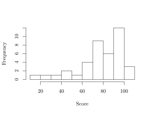
Figure 1 presents a histogram of the data in grades. When I see that distribution, it appears to be a left-skewed distribution. Most students are in the 60-100 range, some scored more than 100, and some scored much less than 60.³ The median grade is 83, the first quartile 71.5, and the third quartile 92. Overall, not a bad distribution that emerged naturally. (No curve was applied.)

If we want to make the grades appear to follow a different distribution, we will need to do the following:

1. Find the percentile of each grade;
2. Find the corresponding distribution of the target distribution; and
3. Replace the original grade at a certain percentile with the corresponding grade from the target distribution.⁴

The following code obtains percentiles:

perc <- (1:length(grades) - 0.5)/length(grades)

Now we need to decide on the target distribution. Supposedly, according to some department chair, grades should be Normally distributed with a mean of a C, which I will take to be 75. That leaves us picking the standard deviation. We probably should pick a standard deviation such that the probability of scoring above 100% is very small; three standard deviations away from the mean should suffice. So we will say that the standard deviation is 9, so .⁵

Let’s now transform grades; to avoid extra controversy, we will also round grades up.

curvegrades <- ceiling(qnorm(perc, mean = 75, sd = 9))

Figure 2: Histogram of curved grades.

Figure 3: Back-to-back stem plots for grades and curvegrades; produced by aplpack::stem.leaf.backback(grades, curvegrades).

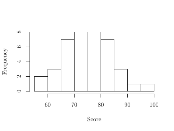
These grades are displayed in Figures 2 and 3. Here are some things to notice from doing this:

• The students in the tail benefited considerably from the curving, gaining considerably and going to D grades when they probably should have failed.
• Most students were penalized by the curve, and in hard-to-understand, seemingly arbitrary ways.
• Only one student will get an A. Another who would have gotten an A got an A-, and several other A students were pushed to the high Bs.

The curve has a very strong effect at the top of the distribution; two students with likely equivalent skill got very different grades, and the student in third place who appears to be just as skilled as the other two if it were not for luck got a B instead of an A. This appears to be very unfair.

Now we could screw around with the parameters and perhaps get a better distribution at the top of the curve, but that raises the question of why any distribution should be forced onto the data, let alone a Normal one. We could just as easily swapped qnorm() with qcauchy() and got a very different distribution for our scores. The data itself doesn’t suggest it came from a Normal distribution, so what makes the Normal distribution special, above all others?

What’s So Special about the Normal Distribution

The Normal distribution has a long history, dating back to the beginning of probability theory. It is the prominent distribution in the Central Limit Theorem and many well-known statistical tests, such at the -test and ANOVA. When people talk about “the bell curve” they are almost always referring to the Normal distribution (there is more than one “bell curve” in probability theory). The Fields Medalist Cédric Villani once said in a 2006 TED talk that if the Greeks had known of the Normal distribution they would have worshipped it like a god.

So why does the Normal distribution hold the place it does? For reference, below is the formula for the PDF of the Normal distribution with mean and variance :

Figure 4: A plot of the PDF of a Normal distribution with mean and variance .

A plot of the Normal distribution is given in Figure 4. At first glance looks complicated, but it’s actually well-behaved and easy to work with. It’s rich in mathematical properties. While in principle any number could be produced by a Normally distributed random variable, in practice seeing anything farther than three standard deviations from the mean is unlikely. It is closed under addition; the sum of two (joinly) Normal random variables is a Normal random variable. And of course it features prominently in the Central Limit Theorem; the sum of IID random variables with finite variance starts to look Normally distributed, and this can happen even when these assumptions are relaxed. Additionally, Central Limit Theorems exists for vectors, functions, and partial sums, and in those cases the limiting distribution is some version of a Normal distribution.

Most practitioners, though, do not appreciate the mathematical “beauty” of the Normal distribution; I doubt this is why people would insist grades should be Normally distributed. Well, perhaps that’s not quite true; people may know that the Normal distribution is special even if they themselves cannot say why, and they may want to see Normal distributions appear to keep with a fad that’s been strong since eugenics. But “fad” feels like a cop-out answer, and I think there are better explanations.⁶

Many people get rudimentary statistical training, and the result is “cargo-cult statistics”, as described by (1);⁷ they practice something that on the surface looks like statistics but lacks true understanding of why the statistical methods work or why certain assumptions were made. People in statistics classes learned about the Normal distribution and their instructors (rightly) drilled its features and its importance into their heads, but the result is that they think data should be Normally distributed since it’s what they know when in reality data can follow any distribution, usually non-Normal ones.

Additionally, statistics’ most popular tests–in particular, the -test and ANOVA–calls for Normally distributed data in order to be applied. And in the defense of practitioners, there are a lot of tests calling for Normally distributed data, especially the ones they learned. But they don’t appreciate why these procedures use the Normal distribution.

The -test and ANOVA, in particular, are some of the oldest tests in existence, being developed by Fisher and Student around the turn of the century, and they prompted a revolution in science. But why did these tests use the Normal distribution? I speculate that a parametric test that worked for Normally distributed data was simply a low-hanging fruit; assuming the data was Normally distributed was the easiest way to produce a meaningful, useful product. Many tests with the same objectives as the -test and ANOVA have been developed that don’t require Normality, but these tests came later and they’re harder to do. (That said, it’s just as easy to do the -test as it is to do an equivalent non-parametric test these days with software, but software is new and also it’s harder to explain what the non-parametric test does to novices.) Additionally, results such as the Central Limit Theorem cause tests requiring Normality to work anyway in large data sets.

Good products often come for Normal things first; generalizations are more difficult and may take more time to be produced and be used. That said, statisticians appreciate the fact that most phenomena is not Normally distributed and that tweaks will need to be made when working with real data. Most people practicing statistics, though, are not statisticians; cargo-cult statistics flourishes.

Conclusion

Since statistics became prominent in science statisticians have struggled with how to handle their own success and most statistics being done by non-statisticians. Statistical education is a big topic since statistics is a hard topic to teach well. Also, failure to understand statistics produces real-world problems, from junk statistics to junk science and policy motivated by it. Assuming grades are Normally distributed is but one aspect of this phenomenon, and one that some students unfortunately feel personally.

Perhaps the first step to dealing with such problems is reading an article like these and appreciating the message. Perhaps it will change an administrator’s mind (but I’m a pessimist). But perhaps the student herself reading this will see the injustice she suffers from such a policy and appreciate why the statisticians are on her side, then commit to never being so irresponsible herself.

Bibliography

1

Philip B. Stark and Andrea Saltelli.
Cargo-cult statistics and scientific crisis.
Significance, 15 (4): 40-43, 2018.
doi: rm10.1111/j.1740-9713.2018.01174.x.
URL https://rss.onlinelibrary.wiley.com/doi/abs/10.1111/j.1740-9713.2018.01174.x.

About this document …

Grades Aren’t Normal

This document was generated using the LaTeX2HTML translator Version 2019 (Released January 1, 2019)

The command line arguments were:
latex2html -split 0 -nonavigation -lcase_tags -image_type gif simpledoc.tex

The translation was initiated on 2019-07-29

Footnotes

… material.¹

This is not the only possible objective of grading. Other grading objectives could be to rate students growth (how much a student improved since the beginning of the class) or to simply say which students were best and which were worst in the class. I take issue personally with either of these alternative “objectives” of grading; the first can be arbitrary and not produce useful information on the student since they could get an “A” for going from “terrible” to “mediocre”, while the second not only suffers from a similar problem (perhaps the “best” student knows little about the material) but also feel elitist.

… distributions.²

Here is an argument for why grades might appear Normally distributed; since a final grade is the sum of grades from assignments, quizzes, tests, and so on, and grades generally emerge from summation of points, we could apply a version of the Central Limit Theorem to argue that the end result should be grades that appear Normally distributed. But there are still assumptions on how strong a dependence there is in points and assignments, and in fact while an individual student’s grades might start to look Normally distributed if such a process were to continue for a long time, this says nothing about the student body since one could say each student is her own data-generating process with her own parameters and those parameters do not follow some larger distribution.

… 60.³

Scoring above 100 is possible in many of the classes I teach due to extra credit opportunities. The low grades are often those belonging to students who have effectively given up on the class, or at least are only moderately connected to it.

… distribution.⁴

In the data set grades, there are ties. This data was rounded; real data would not have such an issue, and presumably an instructor would have access to the original data that wasn’t rounded.

….⁵

I use the variance notation for the Normal distribution; that is, for a Normal random variable with mean and variance .

… explanations.⁶

Tests such as IQ tests and SAT/ACT tests often seem to produce scores following a Normal distribution, but this seems to follow more from construction than from nature. One can see why an educator would start to think that student grades, which also assess “intelligence,” should also be Normally distributed, but this appears to just be accepting a deception.

…starksaltelli18;⁷

The term “cargo-cult” describes a phenomenon observed after the American Pacific campaign of World War II at the islands that once were American bases; island natives would build replicas of the bases and imitate their operations after the military left. They saw and imitated the activities without understanding why they worked. Since then the term has been use to suggest “imitation without understanding;” for example, Nobel physicist Richard Feynman coined the term “cargo-cult science” to mean activity that looks like science but does not honestly apply the scientific method.

Packt Publishing published a book for me entitled Hands-On Data Analysis with NumPy and Pandas, a book based on my video course Unpacking NumPy and Pandas. This book covers the basics of setting up a Python environment for data analysis with Anaconda, using Jupyter notebooks, and using NumPy and pandas. If you are starting out using Python for data analysis or know someone who is, please consider buying my book or at least spreading the word about it. You can buy the book directly or purchase a subscription to Mapt and read it there.

If you like my blog and would like to support it, spread the word (if not get a copy yourself)!