
Expedia Data Analysis Part 1
Want to share your content on R-bloggers? click here if you have a blog, or here if you don't.
Expedia Hotel Recommendations
This dataset can be found at Kaggle. We are given logs of visitors at different Expedia sites and are asked to predict the hotel clusters in the test set. Expedia aims to use customer data to improve their hotel recommendations. In this blog, I will analyze this dataset and try to get some insight of it.
##

Read 37670293 rows and 24 (of 24) columns from 3.791 GB file in 00:02:37

##             used   (Mb) gc trigger   (Mb)  max used   (Mb)
## Ncells  25981347 1387.6   36236006 1935.3  25989623 1388.0
## Vcells 646504616 4932.5 1095841779 8360.7 651377761 4969.7

## Classes 'data.table' and 'data.frame':   37670293 obs. of  24 variables:
##  $ date_time                : chr  "2014-08-11 07:46:59" "2014-08-11 08:22:12" "2014-08-11 08:24:33" "2014-08-09 18:05:16" ...
##  $ site_name                : int  2 2 2 2 2 2 2 2 2 2 ...
##  $ posa_continent           : int  3 3 3 3 3 3 3 3 3 3 ...
##  $ user_location_country    : int  66 66 66 66 66 66 66 66 66 66 ...
##  $ user_location_region     : int  348 348 348 442 442 442 189 189 189 189 ...
##  $ user_location_city       : int  48862 48862 48862 35390 35390 35390 10067 10067 10067 10067 ...
##  $ orig_destination_distance: num  2234 2234 2234 913 914 ...
##  $ user_id                  : int  12 12 12 93 93 93 501 501 501 501 ...
##  $ is_mobile                : int  0 0 0 0 0 0 0 0 0 0 ...
##  $ is_package               : int  1 1 0 0 0 0 0 1 0 0 ...
##  $ channel                  : int  9 9 9 3 3 3 2 2 2 2 ...
##  $ srch_ci                  : chr  "2014-08-27" "2014-08-29" "2014-08-29" "2014-11-23" ...
##  $ srch_co                  : chr  "2014-08-31" "2014-09-02" "2014-09-02" "2014-11-28" ...
##  $ srch_adults_cnt          : int  2 2 2 2 2 2 2 2 2 2 ...
##  $ srch_children_cnt        : int  0 0 0 0 0 0 0 0 0 0 ...
##  $ srch_rm_cnt              : int  1 1 1 1 1 1 1 1 1 1 ...
##  $ srch_destination_id      : int  8250 8250 8250 14984 14984 14984 8267 8267 8267 8267 ...
##  $ srch_destination_type_id : int  1 1 1 1 1 1 1 1 1 1 ...
##  $ is_booking               : int  0 1 0 0 0 0 0 0 0 0 ...
##  $ cnt                      : int  3 1 1 1 1 1 2 1 1 1 ...
##  $ hotel_continent          : int  2 2 2 2 2 2 2 2 2 2 ...
##  $ hotel_country            : int  50 50 50 50 50 50 50 50 50 50 ...
##  $ hotel_market             : int  628 628 628 1457 1457 1457 675 675 675 675 ...
##  $ hotel_cluster            : int  1 1 1 80 21 92 41 41 69 70 ...
##  - attr(*, ".internal.selfref")=

##   date_time           site_name      posa_continent user_location_country
##  Length:37670293    Min.   : 2.000   Min.   :0.00   Min.   :  0.00
##  Class :character   1st Qu.: 2.000   1st Qu.:3.00   1st Qu.: 66.00
##  Mode  :character   Median : 2.000   Median :3.00   Median : 66.00
##                     Mean   : 9.795   Mean   :2.68   Mean   : 86.11
##                     3rd Qu.:14.000   3rd Qu.:3.00   3rd Qu.: 70.00
##                     Max.   :53.000   Max.   :4.00   Max.   :239.00
##
##  user_location_region user_location_city orig_destination_distance
##  Min.   :   0.0       Min.   :    0      Min.   :    0
##  1st Qu.: 174.0       1st Qu.:13009      1st Qu.:  313
##  Median : 314.0       Median :27655      Median : 1140
##  Mean   : 308.4       Mean   :27753      Mean   : 1970
##  3rd Qu.: 385.0       3rd Qu.:42413      3rd Qu.: 2553
##  Max.   :1027.0       Max.   :56508      Max.   :12408
##                                          NA's   :13525001
##     user_id          is_mobile        is_package        channel
##  Min.   :      0   Min.   :0.0000   Min.   :0.0000   Min.   : 0.000
##  1st Qu.: 298910   1st Qu.:0.0000   1st Qu.:0.0000   1st Qu.: 2.000
##  Median : 603914   Median :0.0000   Median :0.0000   Median : 9.000
##  Mean   : 604452   Mean   :0.1349   Mean   :0.2489   Mean   : 5.871
##  3rd Qu.: 910168   3rd Qu.:0.0000   3rd Qu.:0.0000   3rd Qu.: 9.000
##  Max.   :1198785   Max.   :1.0000   Max.   :1.0000   Max.   :10.000
##
##    srch_ci            srch_co          srch_adults_cnt srch_children_cnt
##  Length:37670293    Length:37670293    Min.   :0.000   Min.   :0.0000
##  Class :character   Class :character   1st Qu.:2.000   1st Qu.:0.0000
##  Mode  :character   Mode  :character   Median :2.000   Median :0.0000
##                                        Mean   :2.024   Mean   :0.3321
##                                        3rd Qu.:2.000   3rd Qu.:0.0000
##                                        Max.   :9.000   Max.   :9.0000
##
##   srch_rm_cnt    srch_destination_id srch_destination_type_id
##  Min.   :0.000   Min.   :    0       Min.   :0.000
##  1st Qu.:1.000   1st Qu.: 8267       1st Qu.:1.000
##  Median :1.000   Median : 9147       Median :1.000
##  Mean   :1.113   Mean   :14441       Mean   :2.582
##  3rd Qu.:1.000   3rd Qu.:18790       3rd Qu.:5.000
##  Max.   :8.000   Max.   :65107       Max.   :9.000
##
##    is_booking           cnt          hotel_continent hotel_country
##  Min.   :0.00000   Min.   :  1.000   Min.   :0.000   Min.   :  0.0
##  1st Qu.:0.00000   1st Qu.:  1.000   1st Qu.:2.000   1st Qu.: 50.0
##  Median :0.00000   Median :  1.000   Median :2.000   Median : 50.0
##  Mean   :0.07966   Mean   :  1.483   Mean   :3.156   Mean   : 81.3
##  3rd Qu.:0.00000   3rd Qu.:  2.000   3rd Qu.:4.000   3rd Qu.:106.0
##  Max.   :2.00000   Max.   :269.000   Max.   :6.000   Max.   :212.0
##
##   hotel_market    hotel_cluster
##  Min.   :   0.0   Min.   : 0.00
##  1st Qu.: 160.0   1st Qu.:25.00
##  Median : 593.0   Median :49.00
##  Mean   : 600.5   Mean   :49.81
##  3rd Qu.: 701.0   3rd Qu.:73.00
##  Max.   :2117.0   Max.   :99.00
##
The is_booking and cnt variables are not present in the test
set. And as expected the hotel_cluster variable is also not present
in the test set, as this is the variable to be predicted.
The test set has an ID column, which is not present in the train set.
The ID will be the first column in the submission file, and the
predicted hotel_cluster will be the second. The sample submission file
already has the ID column, thus the ID of test file is not imported.
Let’s convert the types of some columns. is_mobile, is_package,
channel, posa_continent, hotel_continent are categorical variables and
will be converted by using the as.factor function. There are some
other categorical varaibles such as hotel_cluster, hotel_country,
user_location, etc. but these will be left as integer values, since
they have too manyentries, which makes it harder to deal with them when
plotting.
The date columns are imported as characters, and will be converted to
POSIXct date format. The date_time column is the time a search was
made on the website by a user. The year, month, day of week, and day of
month, and hour information will be extracted from the date_time
columns.
I am also making use of garbage collector gc() functions, since I have
realized that when working with big data, there is a lot of leftovers in
the memory which should be cleaned.
trn[, `:=`(is_mobile = as.factor(is_mobile),
               is_package = as.factor(is_package),
               channel = as.factor(channel),
               posa_continent = as.factor(posa_continent),
               hotel_continent = as.factor(hotel_continent))]
gc()


trn[, date_time := parse_date_time(date_time, "%y-%m-%d %H:%M:%S")]
class(trn[,date_time])

## [1] 'POSIXct' 'POSIXt'


trn[, `:=`(date_year = as.factor(year(date_time)),
               date_month = as.factor(month(date_time)),
               date_day = as.factor(day(date_time)),
               date_wday = as.factor(wday(date_time, label = T)),
               date_hour = as.factor(hour(date_time)) )]
gc()
The train dataset has 37,670,293 rows, and 24 columns. This is huge! Now
that we have imported the data and made some conversions, let's start
our analysis.
Exploring the proportion of sites visited reveals that site_name 2 is
the most frequently visited site, which dominates all the others. So, it
has been taken out in the second graph, in order to see other
proportions better.
# barplot site_name
d = trn[, .N, by = site_name][, j = .(site_name, Prop = N/ sum(N))]
g = ggplot(d, aes(x = site_name, y = Prop))
g1 = g + geom_bar(aes(fill = factor(site_name)), stat = 'identity' ) + scale_fill_discrete(name = 'site_name')
ggplotly(g1)

# Site name 2 dominates all the others
d = d[i = site_name != 2]
g = ggplot(d, aes(x = site_name, y = Prop))
g1 = g + geom_bar(aes(fill = factor(site_name)), stat = 'identity') + scale_fill_discrete(name = 'site_name')
ggplotly(g1)

Hotel Cluster – Mobile – Package Relationship
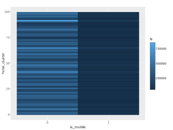
The following graphs are to gain some insight into hotel cluster –
mobile relationship. The majority of customers are not mobile. I use
tile graph where each point is depicted as a rectangle and colored based
on the intensity of the 'fill' value. In this case this is the number of
points falling into each category.
d = trn[,j = .N, by = .(hotel_cluster, is_mobile)]
g = ggplot(d, aes(x = is_mobile, y = hotel_cluster)) + geom_raster(aes(fill = N))
ggplotly(g)
Are there any hotel clusters in which mobile is more prevalent? Instead
of total number at each hotel cluster, it makes more sense to check the
proportions. The proportions are calculated over each hotel_cluster.
Thus, the probabilities in is_mobile0 and is_mobile1 sum up to 1 for
each hotel_cluster.
d = trn[,j = .N, by = .(hotel_cluster, is_mobile)][, Prop := N/ sum(N), by = .(hotel_cluster)]
g = ggplot(d, aes(x = is_mobile, y = hotel_cluster)) + geom_raster(aes(fill = Prop))
ggplotly(g)
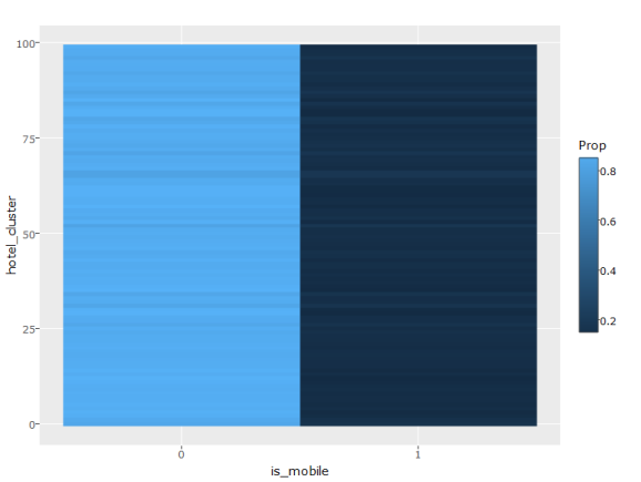
All the hotel_clusters have more or less the same proportion among
is_mobile 0 and 1, with just a few having a larger proportion than
average. Although I like tile graphs, bar graph could be a better
visualization in making a comparison. Let's do that.
d = trn[,j = .N, by = .(hotel_cluster, is_mobile)][, Prop := N/ sum(N), by = .(hotel_cluster)]
g = ggplot(d, aes(x = hotel_cluster, y = Prop)) + geom_bar(aes(fill = Prop), stat = 'identity') + facet_grid(is_mobile~., labeller = label_both)
ggplotly(g)

OK, we see the same here. So no differnce between being mobile or not
and hotel_clusters.
Now, let's check the relation between is_package and hotel_cluster.
Here I have preferred to use the bar plot rather than the tile graph.
d = trn[,j = .N, by = .(hotel_cluster, is_package)]
g = ggplot(d, aes(x = hotel_cluster, y = N)) + geom_bar(aes(fill=factor(hotel_cluster)), stat = 'identity') + facet_grid(is_package~., labeller = label_both)
ggplotly(g)

The above graph tells us that some hotel clusters have more visits. But
in order to see if any hotel cluster is more related to being searched
within a package, we will need to plot the proportions within each
hotel_cluster. In my opinion, some hotel clusters can be related to
being searched within a package deal.
d = trn[,j = .N, by = .(hotel_cluster, is_package)][, Prop := N/ sum(N), by = .(hotel_cluster)]
g = ggplot(d, aes(x = hotel_cluster, y = Prop)) + geom_bar(aes(fill=factor(hotel_cluster)) , stat = 'identity') + facet_grid(is_package~., labeller = label_both) + theme_dark()
ggplotly(g)

Indeed, some clusters such as 52, 65, 66, and 87 are more related to
being in a package.
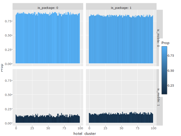
Below I am trying to find a relationship between hotel_cluster, is_mobile, and is_package.
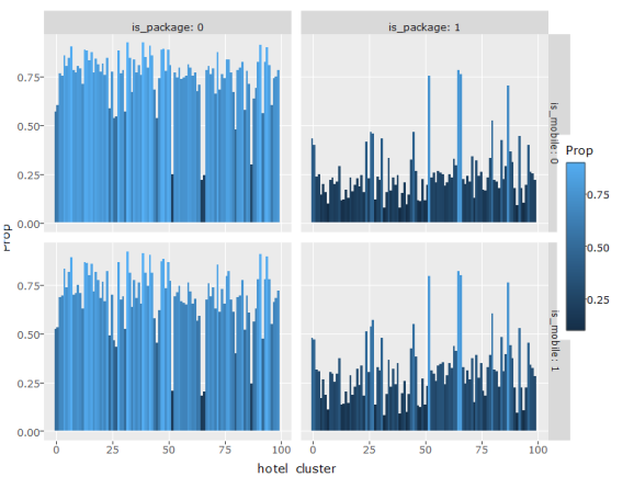
First, when is_mobile is 1, does is_package change or stay the same? As, can be seen, it stays the same, albeit slightly higher proportions of is_package 1 and is_mobile1. Second, when is_package has a large value for a hotel_cluster, does it behave similarly in is_mobile? As can be seen from second graph, is_mobile behaves the same in both of its categories, suggesting indifference to is_package.
d = trn[,j = .N, by = .(hotel_cluster, is_mobile, is_package)][, Prop := N/ sum(N), by = .(hotel_cluster, is_package)]
g = ggplot(d, aes(x = hotel_cluster, y = Prop, fill = Prop))+ geom_bar(stat = 'identity')+facet_grid(is_mobile~is_package, labeller = label_both)
ggplotly(g)
d = trn[,j = .N, by = .(hotel_cluster, is_mobile, is_package)][, Prop := N/ sum(N), by = .(hotel_cluster, is_mobile)]
g = ggplot(d, aes(x = hotel_cluster, y = Prop, fill = Prop))+ geom_bar(stat = 'identity')+facet_grid(is_mobile~is_package, labeller = label_both)
ggplotly(g)
Channel of Marketing
Let's investigate the behavior of marketing channel.
levels(trn$channel)

    ##  "0"  "1"  "2"  "3"  "4"  "5"  "6"  "7"  "8"  "9"  "10"


d = trn[, j = .N, by = .(channel)][, Prop:=N/sum(N)]
g = ggplot(d, aes(x=channel, y= Prop, fill = channel)) + geom_bar(stat = 'identity')
ggplotly(g)

The proportion of channel 9 dominates all the others. Channel 10 is the
least used channel. It makes me wonder whether there is any relation
between channel and being mobile?
d = trn[, j = .N, by = .(is_mobile, channel)][, Prop:=N/sum(N), by = channel]
g = ggplot(d, aes(x = is_mobile, y = channel, fill = Prop)) + geom_raster() + scale_fill_gradient2(name="N", low="blue", mid = 'white' , high="red")
ggplotly(g)

Channel 0, 1 and 2 have larger proportions than average in mobile users,
suggesting that these marketing channels might be a little bit more
geared towards mobile users.
Channel 10, and 6 are interesting as their proportion was very low which
requires further investigation. It might be that Channel 10 and 6 were
unsuccessful and were abandoned after a while. Let's see.
Let's plot months over the two years for channel 9, 6, and 10. For this
I will use the new data extracted from the date field.
d = trn[i = channel == 9, .N, by = .(date_year, date_month)][order(date_year, date_month)]
g = ggplot(d,aes(x= date_month, y = N))+ geom_bar(aes(fill = date_month), stat = 'identity') + facet_grid(date_year~.) + theme(legend.position="none") + ggtitle("Channel 9")
ggplotly(g)

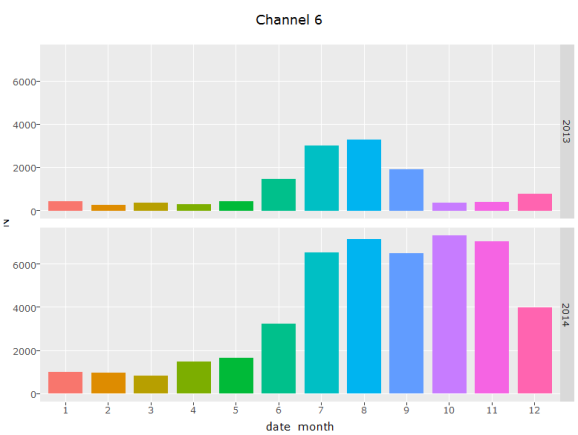
d = trn[i = channel == 6, .N, by = .(date_year, date_month)][order(date_year, date_month)]
g = ggplot(d,aes(x= date_month, y = N, fill = date_month))+ geom_bar(stat = 'identity') + facet_grid(date_year~.) + theme(legend.position="none") + ggtitle("Channel 6")
ggplotly(g)
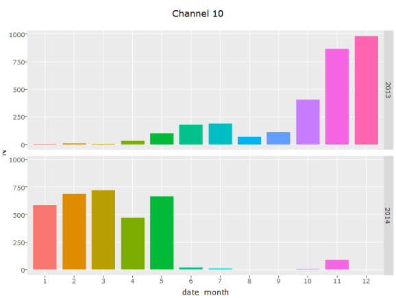
d = trn[i = channel == 10, .N, by = .(date_year, date_month)][order(date_year, date_month)]
g = ggplot(d,aes(x= date_month, y = N, fill = date_month))+ geom_bar(stat = 'identity') + facet_grid(date_year~.) + theme(legend.position="none") + ggtitle("Channel 10")
ggplotly(g)
As can be seen from the tables, I first checked channel 9, which is
distributed over the months in 2013, and 2014. The amount increased by
more than 100% after the first half of 2014.
Channel 6 seems to be a new marketing channel which is seeing some
growth over time. In fact, it has almost quadrupled in the second half
of 2014, compared to January of 2014.
Channel 10 as suspected was tried in 2013 and 2014 but it seems to be a
failure. The numbers are so low, and it seems abandoned after June of
2014. It might also be a very niche market, tried for a little while.
I also have checked all the other marketing channels,and they all behave
almost the same as channel 9. This makes me wonder that ther are amny
more datapoints from 2014, than 2013.
trn[, .N, by = date_year]

##    date_year        N
## 1:      2014 26483412
## 2:      2013 11186881
Indeed, as can be seen there about 11 million points from 2013, and
almost 26.5 million from 2014. This change might be due to the fact the
internet traffic to Expedia is rising by large amounts, and/or simply
more points were sampled from 2014.
Anyway, this is all for now. Hope you gained some insight. I will
analyze the other variables in my second post on this topic. I will also
look further into the trends of different variables. I am curious to see
whether mobile traffic increased from 2013 to 2014.
Please comment below. I am always open to suggestions, and best
practices. Thank you and see you soon!


R-bloggers.com offers daily e-mail updates about R news and tutorials about learning R and many other topics. Click here if you're looking to post or find an R/data-science job.
Want to share your content on R-bloggers? click here if you have a blog, or here if you don't.