
Data Splitting
Want to share your content on R-bloggers? click here if you have a blog, or here if you don't.
A few common steps in data model building are;
- Pre-processing the predictor data (predictor – independent variable’s)
- Estimating the model parameters
- Selecting the predictors for the model
- Evaluating the model performance
- Fine tuning the class prediction rules
“One of the first decisions to make when modeling is to decide which samples will be used to evaluate performance. Ideally, the model should be evaluated on samples that were not used to build or fine-tune the model, so that they provide an unbiased sense of model effectiveness. When a large amount of data is at hand, a set of samples can be set aside to evaluate the final model. The “training” data set is the general term for the samples used to create the model, while the “test” or “validation” data set is used to qualify performance.” (Kuhn, 2013)
In most cases, the training and test samples are desired to be as homogenous as possible. Random sampling methods can be used to create similar data sets. Let’s take an example. I will be using R programming language and will use two datasets from the UCI Machine Learning repository.
# clear the workspace
> rm(list=ls())
# ensure the process is reproducible
> set.seed(2)
The first dataset is the Wisconsin Breast Cancer Database Description: Predict whether a cancer is malignant or benign from biopsy details. Type: Binary Classification Dimensions: 699 instances, 11 attributes Inputs: Integer (Nominal) Output: Categorical, 2 class labels UCI Machine Learning Repository: Description Published accuracy results: Summary
Splitting based on Response/Outcome/Dependent variable
Let’s say, I want to take a sample of 70% of my data, I will do it like
> BreastCancer[sample(nrow(BreastCancer), 524),] # 70% sample size
> table(smpl$Class)
benign malignant
345       179
And when I plot it is shown in figure 1 below;

Figure 1: Plot of categorical class variable
However, if you want to give different probabilities of being selected for the elements, lets say, elements that cancer type is benign has probability 0.25, while those whose cancer type is malignant has prob 0.75, you should do like
> prb <- ifelse(BreastCancer$Class =="benign",0.25, 0.75)
> smpl<- BreastCancer[sample(nrow(BreastCancer), 524, prob = prb),]
> table(smpl$Class)
benign malignant
299     225
And when I plot it is like shown in figure 2,
> plot(smpl$Class)
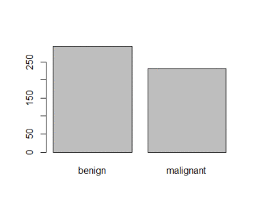 Figure 2: Plot of categorical class variable with probability based sample split If the outcome or the response variable is categorical then split the data using stratified random sampling that applies random sampling within subgroups (such as the classes). In this way, there is a higher likelihood that the outcome distributions will match. The function createDataPartition of the caret package can be used to create balanced splits of the data or random stratified split. I show it using an example in R as given; > library(caret) > train.rows<- createDataPartition(y= BreastCancer$Class, p=0.7, list = FALSE) > train.data<- BreastCancer[train.rows,] # 70% data goes in here > table(train.data$Class) benign malignant 321 169 And the plot shown in figure 3 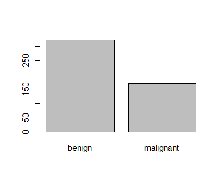 Figure 3: Plot of categorical class variable from train sample data Similarly, I do for the test sample data as given > test.data<- BreastCancer[-train.rows,] # 30% data goes in here > table(test.data$Class) benign malignant 137 72 > plot(test.data$Class) And I show the plot in figure 4,  Figure 4: Plot of categorical class variable from test sample data Splitting based on Predictor/Input/Independent variables So far we have seen the data splitting was based on the outcome or the response variable. However, the data can be split on the predictor variables too. This is achieved by maximum dissimilarity sampling as proposed by Willet (1999) and Clark (1997). This is particularly useful for unsupervised learning where there are no response variables. There are many methods in R to calculate dissimilarity. caret uses the proxy package. See the manual for that package for a list of available measures. Also, there are many ways to calculate which sample is “most dissimilar”. The argument obj can be used to specify any function that returns a scalar measure. caret includes two functions, minDiss and sumDiss, that can be used to maximize the minimum and total dissimilarities, respectfully. References Kuhn, M.,& Johnson, K. (2013). Applied predictive modeling (pp. 389-400). New York: Springer. Willett, P. (1999), “Dissimilarity-Based Algorithms for Selecting Structurally Diverse Sets of Compounds,” Journal of Computational Biology, 6, 447-457.
R-bloggers.com offers daily e-mail updates about R news and tutorials about learning R and many other topics. Click here if you're looking to post or find an R/data-science job.
Want to share your content on R-bloggers? click here if you have a blog, or here if you don't.