A simple Metropolis-Hastings MCMC in R
Want to share your content on R-bloggers? click here if you have a blog, or here if you don't.
While there are certainly good software packages out there to do the job for you, notably BUGS or JAGS, it is instructive to program a simple MCMC yourself. In this post, I give an educational example of the Bayesian equivalent of a linear regression, sampled by an MCMC with Metropolis-Hastings steps, based on an earlier version which I did to together with Tamara Münkemüller. Since first publishing this post, I have made a few small modifications to improve clarity. A similar post on Metropolis-Hastings MCMC algorithms by Darren Wilkinson is also worth looking at. Also, we give an introduction on this algorithm and alternatives in our review on statistical inference for stochastic simulation models. [Update]: More on analyzing the results of this algorithm can be found in a recent post.
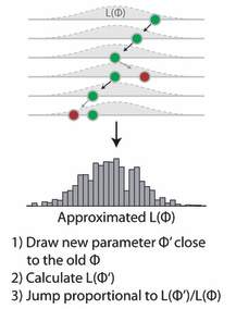
Figure: A visualization of the Metropolis-Hastings MCMC, from Hartig et al., 2011. (copyright see publisher)
Creating test data
As a first step, we create some test data that will be used to fit our model. Let’s assume a linear relationship between the predictor and the response variable, so we take a linear model and add some noise.
# This work is licensed under the Creative Commons Attribution-NonCommercial-ShareAlike 3.0 Unported License.

trueA <- 5
trueB <- 0
trueSd <- 10
sampleSize <- 31

# create independent x-values
x <- (-(sampleSize-1)/2):((sampleSize-1)/2)
# create dependent values according to ax + b + N(0,sd)
y <-  trueA * x + trueB + rnorm(n=sampleSize,mean=0,sd=trueSd)

plot(x,y, main="Test Data")
I balanced x values around zero to “de-correlate” slope and intercept. The result should look something like the figure to the right
Defining the statistical model
The next step is to specify the statistical model. We already know that the data was created with a linear relationship y = a*x + b between x and y and a normal error model N(0,sd) with standard deviation sd, so let’s use the same model for the fit and see if we can retrieve our original parameter values.
Derive the likelihood function from the model
For estimating parameters in a Bayesian analysis, we need to derive the likelihood function for the model that we want to fit. The likelihood is the probability (density) with which we would expect the observed data to occur conditional on the parameters of the model that we look at. So, given that our linear model y = b + a*x + N(0,sd) takes the parameters (a, b, sd) as an input, we have to return the probability of obtaining the test data above under this model (this sounds more complicated as it is, as you see in the code, we simply calculate the difference between predictions y = b + a*x and the observed y, and then we have to look up the probability densities (using dnorm) for such deviations to occur.
likelihood <- function(param){
	a = param[1]
	b = param[2]
	sd = param[3]

	pred = a*x + b
	singlelikelihoods = dnorm(y, mean = pred, sd = sd, log = T)
	sumll = sum(singlelikelihoods)
	return(sumll)
}

# Example: plot the likelihood profile of the slope a
slopevalues <- function(x){return(likelihood(c(x, trueB, trueSd)))}
slopelikelihoods <- lapply(seq(3, 7, by=.05), slopevalues )
plot (seq(3, 7, by=.05), slopelikelihoods , type="l", xlab = "values of slope parameter a", ylab = "Log likelihood")
As an illustration, the last lines of the code plot the Likelihood for a range of parameter values of the slope parameter a. The result should look something like the plot to the right.
Why we work with logarithms
You might have noticed that I return the logarithm of the probabilities in the likelihood function, which is also the reason why I sum the probabilities of all our datapoints (the logarithm of a product equals the sum of the logarithms). Why do we do this? You don’t have to, but it’s strongly advisable because likelihoods, where a lot of small probabilities are multiplied, can get ridiculously small pretty fast (something like 10^-34). At some stage, computer programs are getting into numerical rounding or underflow problems then. So, bottom-line: when you program something with likelihoods, always use logarithms!!!
Defining the prior
As a second step, as always in Bayesian statistics, we have to specify a prior distribution for each parameter. To make it easy, I used uniform distributions and normal distributions for all three parameters. [Some additional information for the "professionals", skip this when you don't understand what I'm talking about: while this choice can be considered pretty "uninformative" for the slope and intercept parameters, it is not really uninformative for the standard deviations. An uninformative prior for the latter would usually be scale with 1/sigma (if you want to understand the reason, see here). This stuff is important when you seriously dive into Bayesian statistics, but I didn't want to make the code more confusing here.]
# Prior distribution
prior <- function(param){
	a = param[1]
	b = param[2]
	sd = param[3]
	aprior = dunif(a, min=0, max=10, log = T)
	bprior = dnorm(b, sd = 5, log = T)
	sdprior = dunif(sd, min=0, max=30, log = T)
	return(aprior+bprior+sdprior)
}
The posterior
The product of prior and likelihood is the actual quantity the MCMC will be working on. This function is called the posterior (or to be exact, it’s called the posterior after it’s normalized, which the MCMC will do for us, but let’s not be picky for the moment). Again, here we work with the sum because we work with logarithms.
posterior <- function(param){
   return (likelihood(param) + prior(param))
}
The MCMC
Now, here comes the actual Metropolis-Hastings algorithm. One of the most frequent applications of this algorithm (as in this example) is sampling from the posterior density in Bayesian statistics. In principle, however, the algorithm may be used to sample from any integrable function. So, the aim of this algorithm is to jump around in parameter space, but in a way that the probability to be at a point is proportional to the function we sample from (this is usually called the target function). In our case this is the posterior defined above.
This is achieved by
- Starting at a random parameter value
- Choosing a new parameter value close to the old value based on some probability density that is called the proposal function
- Jumping to this new point with a probability p(new)/p(old), where p is the target function, and p>1 means jumping as well
It’s fun to think about why that works, but for the moment I can assure you it does – when we run this algorithm, distribution of the parameters it visits converges to the target distribution p. So, let’s get this in R:
######## Metropolis algorithm ################

proposalfunction <- function(param){
	return(rnorm(3,mean = param, sd= c(0.1,0.5,0.3)))
}

run_metropolis_MCMC <- function(startvalue, iterations){
	chain = array(dim = c(iterations+1,3))
	chain[1,] = startvalue
	for (i in 1:iterations){
		proposal = proposalfunction(chain[i,])

		probab = exp(posterior(proposal) - posterior(chain[i,]))
		if (runif(1) < probab){
			chain[i+1,] = proposal
		}else{
			chain[i+1,] = chain[i,]
		}
	}
	return(chain)
}

startvalue = c(4,0,10)
chain = run_metropolis_MCMC(startvalue, 10000)

burnIn = 5000
acceptance = 1-mean(duplicated(chain[-(1:burnIn),]))
Again, working with the logarithms of the posterior might be a bit confusing at first, in particular when you look at the line where the acceptance probability is calculated (probab = exp(posterior(proposal) – posterior(chain[i,]))). To understand why we do this, note that p1/p2 = exp[log(p1)-log(p2)].
The first steps of the algorithm may be biased by the initial value, and are therefore usually discarded for the further analysis (burn-in time). An interesting output to look at is the acceptance rate: how often was a proposal rejected by the metropolis-hastings acceptance criterion? The acceptance rate can be influenced by the proposal function: generally, the closer the proposals are, the larger the acceptance rate. Very high acceptance rates, however, are usually not beneficial: this means that the algorithms is “staying” at the same point, which results in a suboptimal probing of the parameter space (mixing). It can be shown that acceptance rates between 20% and 30% are optimal for typical applications (more on that here).
Finally, we can plot the results. There are more elegant ways of plotting this which I discuss in another recent post, so check this out, but for the moment I didn’t want to use any packages, so we do it the hard way:
### Summary: #######################

par(mfrow = c(2,3))
hist(chain[-(1:burnIn),1],nclass=30, , main="Posterior of a", xlab="True value = red line" )
abline(v = mean(chain[-(1:burnIn),1]))
abline(v = trueA, col="red" )
hist(chain[-(1:burnIn),2],nclass=30, main="Posterior of b", xlab="True value = red line")
abline(v = mean(chain[-(1:burnIn),2]))
abline(v = trueB, col="red" )
hist(chain[-(1:burnIn),3],nclass=30, main="Posterior of sd", xlab="True value = red line")
abline(v = mean(chain[-(1:burnIn),3]) )
abline(v = trueSd, col="red" )
plot(chain[-(1:burnIn),1], type = "l", xlab="True value = red line" , main = "Chain values of a", )
abline(h = trueA, col="red" )
plot(chain[-(1:burnIn),2], type = "l", xlab="True value = red line" , main = "Chain values of b", )
abline(h = trueB, col="red" )
plot(chain[-(1:burnIn),3], type = "l", xlab="True value = red line" , main = "Chain values of sd", )
abline(h = trueSd, col="red" )

# for comparison:
summary(lm(y~x))
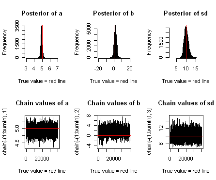
The resulting plots should look something like the plot below. You see that we retrieve more or less the original parameters that were used to create our data, and you also see that we get a certain area around the highest posterior values that also have some support by the data, which is the Bayesian equivalent of confidence intervals.
Figure: The upper row shows posterior estimates for slope (a), intercept (b) and standard deviation of the error (sd). The lower row shows the Markov Chain of parameter values.
Gelman, A.; Carlin, J. B.; Stern, H. S. & Rubin, D. B. (2003) Bayesian Data Analysis
Andrieu, C.; de Freitas, N.; Doucet, A. & Jordan, M. I. (2003) An introduction to MCMC for machine learning Mach. Learning, Springer, 50, 5-43
R-bloggers.com offers daily e-mail updates about R news and tutorials about learning R and many other topics. Click here if you're looking to post or find an R/data-science job.
Want to share your content on R-bloggers? click here if you have a blog, or here if you don't.


