To Difference or Not To Difference?
Want to share your content on R-bloggers? click here if you have a blog, or here if you don't.
In the textbook of time series analysis, we’ve been taught to difference the time series in order to have a stationary series, which can be justified by various plots and statistical tests.
In the real-world time series analysis, things are not always as clear as shown in the textbook. For instance, although the ACF plot shows a not-so-slow decay pattern, ADF test however can’t reject the null hypothesis of a unit root. In such cases, many analysts might tend to difference the time series to be on the safe side in their view.
However, is it really a safe practice to difference a time series anyway to have a stationary series to model? In the example below, I will show that inappropriately differencing a time series would lead the model development to an undesirable direction.
First of all, let’s simulate an univariate series under the Gaussian distributional assumption. By theory, this series has to be stationary.
> library(urca)
> library(forecast)
> library(normwhn.test)
> x <- rnorm(100)
> par(mfrow = c(2, 1))
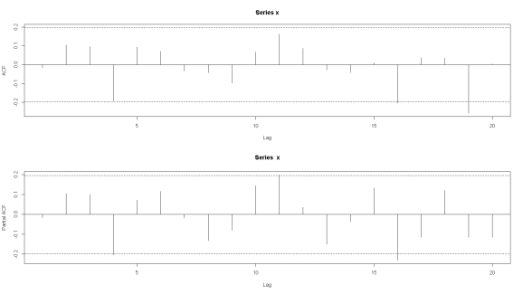
> acf(x)
> pacf(x)
> whitenoise.test(x)
[1] "no. of observations"
[1] 100
[1] "T"
[1] 50
[1] "CVM stat MN"
[1] 0.8687478
[1] "tMN"
[1] -0.9280931
[1] "test value"
[1] 0.6426144
> x.adf <- ur.df(x, type = c("none"), selectlags = "BIC")
> summary(x.adf)

###############################################
# Augmented Dickey-Fuller Test Unit Root Test #
###############################################

Test regression none


Call:
lm(formula = z.diff ~ z.lag.1 - 1 + z.diff.lag)

Residuals:
     Min       1Q   Median       3Q      Max
-1.75385 -0.60585 -0.03467  0.61702  3.10100

Coefficients:
            Estimate Std. Error t value Pr(>|t|)
z.lag.1    -1.008829   0.143635  -7.024  3.1e-10 ***
z.diff.lag  0.002833   0.101412   0.028    0.978
---
Signif. codes:  0 ‘***’ 0.001 ‘**’ 0.01 ‘*’ 0.05 ‘.’ 0.1 ‘ ’ 1

Residual standard error: 0.9501 on 96 degrees of freedom
Multiple R-squared:  0.5064,    Adjusted R-squared:  0.4961
F-statistic: 49.25 on 2 and 96 DF,  p-value: 1.909e-15

Value of test-statistic is: -7.0235

Critical values for test statistics:
     1pct  5pct 10pct
tau1 -2.6 -1.95 -1.61

> x.pkss <- ur.kpss(x, type = "mu", lags = "short")
> summary(x.pkss)

#######################
# KPSS Unit Root Test #
#######################

Test is of type: mu with 4 lags.

Value of test-statistic is: 0.4136

Critical value for a significance level of:
                10pct  5pct 2.5pct  1pct
critical values 0.347 0.463  0.574 0.739

> auto.arima(x, ic = 'bic')
Series: x
ARIMA(0,0,0) with zero mean

sigma^2 estimated as 0.8829:  log likelihood=-135.67
AIC=273.34   AICc=273.38   BIC=275.94
As shown in the above output:
1) Since x is simulated with the normal assumption, the series should be a white noise by definition.
2) ACF plot shows no auto-correlation at all, as it should.
3) In ADF test, the null hypothesis of unit root is rejected.
4) In PKSS test, the null hypothesis of stationarity is not rejected.
5) The output from auto.arima() suggests an ARIMA(0, 0, 0) model, which is completely in line with the assumption.
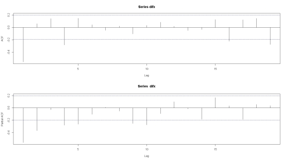
However, what would happen if we take the difference of x anyway?

> difx <- diff(x)
> par(mfrow = c(2, 1))
> acf(difx)
> pacf(difx)
> whitenoise.test(difx)
[1] "no. of observations"
[1] 99
[1] "T"
[1] 49
[1] "CVM stat MN"
[1] 1.669876
[1] "tMN"
[1] 4.689132
[1] "test value"
[1] 0.01904923
> auto.arima(difx, ic = 'bic')
Series: difx
ARIMA(0,0,1) with zero mean

Coefficients:
          ma1
      -0.9639
s.e.   0.0327

sigma^2 estimated as 0.901:  log likelihood=-136.64
AIC=277.27   AICc=277.4   BIC=282.46
The above output is quite interesting in a way that we just artificially “created” a model by over-differencing the white noise series.
1) After over-differenced, the series is not a white noise anymore with the null hypothesis rejected, e.g. p-value = 0.02.
2) In addition, the auto.arima() suggests that an ARIMA(0, 0, 1) model might fit the data.
R-bloggers.com offers daily e-mail updates about R news and tutorials about learning R and many other topics. Click here if you're looking to post or find an R/data-science job.
Want to share your content on R-bloggers? click here if you have a blog, or here if you don't.

